Measuring the impact of technological innovation, green energy, and sustainable development on the health system performance and human well-being: Evidence from a machine learning-based approach

Alaeddine Mihoub; Montassar Kahia; Mohannad Alswailim; Alaeddine Mihoub; Montassar Kahia; Mohannad Alswailim

doi:10.3934/environsci.2024035

AIMS Environmental Science

2024, Volume 11, Issue 5: 703-722. doi: 10.3934/environsci.2024035

Previous Article Next Article

Research article Special Issues

Measuring the impact of technological innovation, green energy, and sustainable development on the health system performance and human well-being: Evidence from a machine learning-based approach

1.
Department of Management Information Systems, College of Business and Economics, Qassim University, Saudi Arabia
2.
Department of Economics, College of Business and Economics, Qassim University, Saudi Arabia

Received: 23 June 2024 Revised: 05 August 2024 Accepted: 22 August 2024 Published: 27 August 2024

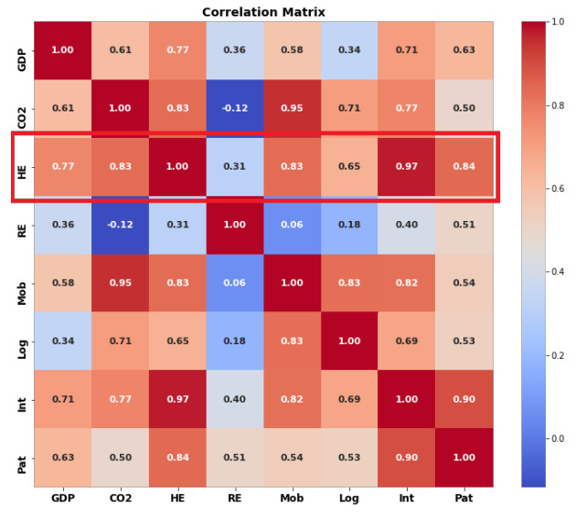
Health performance and well-being are crucial elements of Saudi Arabia's Vision 2030, aiming to improve the overall quality of life and promote a prosperous community. Within this context, this study intended to examine the impact of recent innovations, logistical measures, Information and Communication Technology (ICT) diffusion, environmental quality improvements, economic growth, and green (renewable) energy exploitation on health performance and well-being, in Saudi Arabia from 1990 to 2022, by implementing machine learning models (random forest and gradient boosting) and regression algorithms (ridge and lasso). Overall, the findings of machine learning models indicate a strong impact of digital connectivity on health spending by internet users, with scores of 0.673 and 0.86. Further, economic growth also influences health costs but to a lesser extent, with scores of 0.145 and 0.082. Mobile user penetration and CO₂ emissions have moderate to low importance, suggesting nuanced interactions with health expenditure. Patent applications and logistics performance show minimal impact, indicating a limited direct influence on health costs within this study. Similarly, the share of renewable energy is negligible, reflecting its minimal impact on the analyzed data. Finally, regression analyses using ridge and lasso models confirmed similar trends, further validating these findings. Limitations and several policy implications are also debated.

Keywords:

Citation: Alaeddine Mihoub, Montassar Kahia, Mohannad Alswailim. Measuring the impact of technological innovation, green energy, and sustainable development on the health system performance and human well-being: Evidence from a machine learning-based approach[J]. AIMS Environmental Science, 2024, 11(5): 703-722. doi: 10.3934/environsci.2024035

Related Papers:

[1]	G. Nandini, M. Venkatachalam, Raúl M. Falcón . On the r-dynamic coloring of subdivision-edge coronas of a path. AIMS Mathematics, 2020, 5(5): 4546-4562. doi: 10.3934/math.2020292
[2]	Meiqin Jin, Ping Chen, Shuangliang Tian . Interval edge colorings of the generalized lexicographic product of some graphs. AIMS Mathematics, 2024, 9(11): 30597-30611. doi: 10.3934/math.20241477
[3]	T. Deepa, M. Venkatachalam, Raúl M. Falcón . On the r-dynamic coloring of the direct product of a path with either a path or a cycle. AIMS Mathematics, 2020, 5(6): 6496-6520. doi: 10.3934/math.2020419
[4]	Shuangliang Tian, Ping Chen . Edge-coloring of generalized lexicographic product of graphs. AIMS Mathematics, 2024, 9(6): 15988-15995. doi: 10.3934/math.2024774
[5]	Syed Ahtsham Ul Haq Bokhary, Zill-e-Shams, Abdul Ghaffar, Kottakkaran Sooppy Nisar . On the metric basis in wheels with consecutive missing spokes. AIMS Mathematics, 2020, 5(6): 6221-6232. doi: 10.3934/math.2020400
[6]	Gaixiang Cai, Fengru Xiao, Guidong Yu . The identification numbers of lollipop graphs. AIMS Mathematics, 2025, 10(4): 7813-7827. doi: 10.3934/math.2025358
[7]	Kiki A. Sugeng, Fery Firmansah, Wildan, Bevina D. Handari, Nora Hariadi, Muhammad Imran . Several properties of antiadjacency matrices of directed graphs. AIMS Mathematics, 2024, 9(10): 27834-27847. doi: 10.3934/math.20241351
[8]	Yanyi Li, Lily Chen . Injective edge coloring of generalized Petersen graphs. AIMS Mathematics, 2021, 6(8): 7929-7943. doi: 10.3934/math.2021460
[9]	Shahbaz Ali, Muhammad Khalid Mahmmod, Raúl M. Falcón . A paradigmatic approach to investigate restricted hyper totient graphs. AIMS Mathematics, 2021, 6(4): 3761-3771. doi: 10.3934/math.2021223
[10]	Hongyu Chen, Li Zhang . A smaller upper bound for the list injective chromatic number of planar graphs. AIMS Mathematics, 2025, 10(1): 289-310. doi: 10.3934/math.2025014

Abstract

1. Introduction

The number of studies and discussions in terms of sustainable supply chain management (SSCM) has been increasing rapidly in recent years. As a result, emerged concepts related to sustainability, such as sustainable production and sustainable development, have gradually become more popular globally under various industries ^[1,2]. Incredibly, although it is easier to focus on the manufacturers and assess their efforts towards sustainability by eco-friendly products, conducted sustainability standards ^[1,3]. It is nevertheless clear that the SSCM can only be obtained by the contributions of all stakeholders in the supply chain consist of suppliers or customers ^[4]. In recent years, managers' cognition has been changed in this regard. In general, all issues related to the natural environment, community, or financial benefits are carefully considered under global competitive conditions ^[5,6]. Consequently, several scholars believed that the top management should integrate sustainability philosophy into business strategies to solve the pressures from stakeholders ^[3,7]. The evolution of the sustainability philosophy has influenced the organizations' development strategy. Some recent studies documented that under different research contexts would identify various parameters as well as barriers ^[1,8]. Such as, Zimon et al. (2020) have highlighted various drivers and barriers for the SSCM through the conditions of seventeen Sustainable Development Goals (SDGs) of the United Nations ^[2]. Combination employing ISM and AHP approach to pointed out twenty most essential factors of the SSCM by the Indian engine sector ^[9]. In the Iranian mining industries, forty-one SSCM barriers have been identified ^[10]. Besides, the different research methods of the scholars will also present inconsistent findings related to the parameters' importance, such as Delphi technique ^[7,11]; ISM approach ^[3,12]; or conducting simultaneously two techniques to address research objectives ^[8,9]. Thus, it is clear that these diversities have suggested many promising future research gaps for other scholars to be concerned with the SSCM practice topic in identifying the prevailing parameters.

In Taiwan, numerous sustainability initiatives have been discussed and widely adopted in the various supply chains ^[13]. However, most studies only focus on Taiwan's vital industries, such as semiconductor manufacturing or electronics assembly ^[13,14]. Lack of research about the SSCM of agriculture sectors; meanwhile, the agricultural industries have great significance to the households of indigenous people, especially in rural areas ^[15]. Besides, several sustainable development policies have been published to improve the livelihood of that community group ^[16]. Recently, Taiwan's fresh fruit export industry is seriously affected by import bans from the Chinese market, and the total expected export value will be reduced by twenty percent in 2021 ^[17]. Thereby, this problem has a significant impact on Taiwan's fruit supply chain, particularly affecting farmers' livelihoods. Besides, excessive dependence on one market has seriously affected the sustainability of this supply chain. Thus, forcing Taiwan's fruit supply chain to change to ensure sustainability. According to the existing literature on the sustainable supply chain management topic, the authors aim to identify which essential parameters are given the attention and effect on the SSCM of the industry. Therefore, the Taiwanese fresh-fruit sector has been chosen for practical research to examine which parameters must be considered. This article aims to solve research objectives as follows: RO1. Identification of critical parameters for SSCM under the Taiwanese fresh-fruit sector; RO2. Evaluation to identify the most significant SSCM parameters in this context.

Concentrating on the discussion in parameters contribute to the Taiwanese sustainable fresh-fruit supply chain context as a unique research and promising. The Technique for Order of Preference by Similarity to Ideal Solution (TOPSIS) is one of the multi-criteria decision-making methods and is an outstanding technique to widely conducted ^[4]. Its ability has an excellent quality to solve complex problems and evaluate the importance of parameters ^[4,18]. Thereby, to solve two research objectives that this manuscript would conduct the TOPSIS tool to present the most significant SSCM parameters by the empirical research in Taiwan. Hence, this study would reveal some new methodological insights that bridge academia and practice for SSCM regard. Importantly, the research findings will contribute several theoretical implications for the SSCM literature. Besides, it would suggest some suggestions for managers several practical implications in this regard.

2. Literature review

2.1. Research gaps

The existing literature recently revealed that the SSCM implementation topic had gained significant discussion in academics and practices thanks to the positive impact of sustainability in order to enhance business performance ^[2,19]. Although there are still controversial discussions about the definition of SSCM; however, most scholars agree that the SSCM implementation is in line with the economic, social, and environmental considerations to making business strategies ^[2,8]. Several recent studies indicated that under different research contexts would identify various parameters and barriers ^[1]. The examples can be Narimissa et al. (2020) suggested ten drivers and barrier to implement SSCM in the Iranian oil sector ^[7]. Consistent with that, Zimon et al. (2020) proposed the model for conducting SDGs in the SSCM ^[2]. After that, Pandey et al. (2021) employed the hybrid method to pointed out twenty most essential factors of the SSCM by the Indian engine sector ^[9]. Hence, these studies suggested promising future research gaps for other scholars to be concerned with the SSCM practice topic in identifying the prevailing parameters.

Furthermore, to determine the research gaps and identify the critical variables for SSCM; hence, the authors collect all papers related to SSCM practices and relevant impact elements based on the WoS and SCOPUS database. Several keywords for searching include "sustainable"; "supply chain management"; "parameter"; "barriers"; "elements"; "critical factors". As a result, a total of thirty-one journal papers have been assembled. They are discussed in various contexts, such as nations, industries, and approaches. A systematic analysis of all previous studies on the SSCM implementation topic has been conducted (presented Figure 1). The research gaps are identified in the following points relying on the existing SSCM implementation studies.

Figure 1. Analysis of co-occurrence of author keywords.

DownLoad: Full-Size Img PowerPoint

Firstly, the SSCM literature has witnessed the lack of empirical research in Taiwan, especially agriculture sector ^[13,14]; meanwhile, developing nations are the most preferred research context, for instance, India (n = 10) and China (n = 4). This is the first empirical research in Taiwanese food industry for the SSCM practices regard.

Secondly, sustainability studies regarding supply chain management have focused mainly on manufacturing, while the agricultural sector has experienced no specific research. Moreover, Taiwan's economy was well-known by the semiconductor manufacturing industry ^[14]; thus, conducting the study for the fresh-fruit supply chain has a significant impact on Taiwan's sustainable development, notably would broaden the SSCM practices literature in various sectors.

Thirdly, in terms of research method conducted, the majority of documents prioritize employed qualitative methods, such as ISM (n = 9) and Delphi (n = 6). However, the existing literature does not record any studies that have conducted the TOPSIS approach to consider this issue. Besides, some researchers proposed the TOPSIS as an outstanding technique, its ability is deemed good-quality to solve complex problems and enough to evaluate the importance of elements ^[4,18]. Hence, conducting the TOPSIS technique in this study would offer some new methodological insights that bridge academia and practice for SSCM regard.

2.2. Identification the critical parameters of SSCM

According to the existing sustainability literature about supply chain management, twelve critical parameters reported to contribute to SSCM practices are demonstrated in Table 1.

Table 1. Identification the Critical Parameters of SSCM.

Coding	Parameters	Brief Description	Sources
P1	Planning & Implementation	The optimal design of the fresh fruit supply chain is inevitable, and it requires proper planning and implementation.	^{[4,7,20,21,22]}
P2	Knowledge & Training of fruit preservation	The preservation of post-harvest products needs to apply the latest knowledge and disseminate it to the stakeholders of the chain, particularly in farms and micro corporates.	^[4,23,24,25]
P3	Farming area/ farmer	As the first stage of the food supply chain, the essential role of farms to provide fresh products to the wholesalers, factories, and end customers.	^{[5,15,26,27,28]}
P4	Processing & Packaging	Fresh products need to maintain optimum quality for the longest time. Therefore, standardization and synchronization of processing and packaging must be attention for all the stages.	^{[4,20,29,30,31]}
P5	Warehouse/Storage	Warehouse acts as a transit station in the middle of the food supply chain, the quality of products will be significantly affected by storage operation in warehouses.	^{[18,24,30,32]}
P6	Distribution & Logistics service	The smooth flow of goods in the food supply chain will depend heavily on distribution channels and logistics services.	^[5,18,33,34]
P7	Product quality & Safety	Fresh goods have stringent requirements for standard product quality and safety. It is the participation of the whole chain and must be guaranteed from the stage of planting and harvesting to the end stage.	^[4,35,36]
P8	Contracting	Offering a variety of contracts for choose to ensure the benefits of each counterpart in the food supply chain. Thereby, it helps to reduce risks and conflicts among members.	^{[12,18,37,38]}
P9	Technology adoption	Adopting the latest technology to the supply chain is part of the stakeholders' efforts to obtain sustainability, such as minimizing the impact on the natural environment, reducing costs.	^[39,40,41]
P10	Customer	As the end-stage in the supply chain and consume products, the perceptions and reactions of this group is the driver and will significantly impact the sustainability initiatives of other stakeholders.	^{[20,34,42,43]}
P11	Organizational social responsibilities	Conducting social programs for the local communities has been launched in the sustainable development goals. Forcing the various organization to perform.	^[1,21,44,45]
P12	Collaboration	Collaboration among supply chain members would reinforce sustainability and obtain better performance by reducing financial constraints and production scale.	^{[5,6,31,46,47]}.

| Show Table

DownLoad: CSV

3. Research methodology

3.1. TOPSIS approach

Pointing out optimal solutions according to various parameter selections, these results can be a resource to refer to before decision-making in many different practice situations. The authors assemble data through surveying with ten professionals in the SSCM expertise. They would play the role of decision-makers relying on their experience and knowledge. Collecting data has been done based on twelve clarified SSCM parameters. Employing the TOPSIS approach analyzes the expert's response to solving the second research objective.

The authors can rank all SSCM parameters to determine the most significant variables for the current Taiwanese fresh-fruit supply chain. In this study, ten experts in the Taiwanese fresh-fruit supply chain were asked to rate all criteria. The language terms will be defined from 1 to 10; in detail, "1" means "Extremely unimportant", and "10" means "Extremely important". Consequently, the TOPSIS algorithm could be conducted by the following process:

Step one: Relying on m alternative and n criteria having a rating of i^th decision-makers and j^th criteria. A matrix format as ${{\text{[}}{x_{ij}}{\text{]}}_{m*n}}$ can be expressed for a MCDM issues as below.

$\left\{ \begin{array}{l} {x_{11}}{x_{12}}......{x_{1n}} \\ {x_{21}}{x_{22}}......{x_{2n}} \\ . \\ . \\ {x_{m1}}{x_{m2}}......{x_{mn}} \end{array} \right\} i = 1, 2, ..., m ; j = 1, 2, ... , n$

Step two: The normalize decision matrix has been calculated in Eq 1, where i = 1, 2, ..., n; and j = 1, 2, ..., m. And then, obtaining the normalized decision matrix by calculate the value ${{{r}}_{ij}}$ .

${r_{ij}} = \frac{{x_{ij}^{}}}{{\sqrt {\sum\limits_{i = 1}^n {x_{ij}^2} } }}$

(1)

$\left\{ \begin{array}{l} {r_{11}}{r_{12}}......{r_{1n}} \\ {r_{21}}{r_{22}}......{r_{2n}} \\ . \\ . \\ {r_{m1}}{r_{m2}}......{r_{mn}} \end{array} \right\}$

Step three: The authors then construct the weighted normalized matrix by calculate ${{{v}}_{ij}}$ .

${v_{ij}} = {{\text{w}}_j}*{{\text{r}}_{ij}}$

(2)

$\left\{ \begin{array}{l} {v_{11}}{v_{12}}......{v_{1n}} \\ {v_{21}}{v_{22}}......{v_{2n}} \\ . \\ . \\ {v_{m1}}{v_{m2}}......{v_{mn}} \end{array} \right\}$

In details, w_j = weights of different attributes; (i = 1, 2, …, n; j = 1, 2, …, m)

Step four: Identifying the ideal solution consist of positive ideal solution (A⁺) and negative ideal solution (A^-), the distance of these ideal solutions has been revealed by maximum and minimize value as below.

${A^ + } = \left( {v_1^ + , v_2^ + , ..., v_n^ + } \right) \;\;\; {\rm{with}} \;\;\;\;{v_j}^ + = \left\{ {\max {x_i}.{v_{ij}}, {{\min }_i}.{v_{ij}}} \right\}$

(3)

${A^ - } = \left( {v_1^ - , v_2^ - , ..., v_n^ - } \right) \;\;\;\;{\rm{with}} \;\;\;\;{v_j}^ - = \left\{ {{{\min }_i}.{v_{ij}}, \max {x_i}.{v_{ij}}} \right\}$

(4)

Step five: Determining each alternative's distance by calculating the Euclidean distance from the positive and negative ideal solutions. Those solutions are calculated by two values as $s_i^ +$ and $s_i^ -$ , and can be shown in Eqs 5 and 6, respectively.

$s_i^ + = \sqrt {\sum\limits_j {{{\left( {v_{ij}^ + - v_j^ + } \right)}^2}} }$

(5)

$s_i^ - = \sqrt {\sum\limits_j {{{\left( {v_{ij}^ - - v_j^ - } \right)}^2}} }$

(6)

with i = 1, 2, ..., m and j = 1, 2, ..., n.

Step six: The authors calculate the closeness coefficient values (CC_i) of each alternative by the Eq 7:

$C{C_i} = \frac{{s_i^ - }}{{s_i^ - + s_i^ + }} \;\;\;\; {\rm{with}}\; i = 1, 2, ..., {\rm{m}}$

(7)

Step seven: Determining the optimal solutions according to the CC_i values range from 0 to 1 scale, the great solution according to the alternative value closest to 1 cutoff. Further, the authors also can determine exactly the rank of these alternatives thanks to these CC_i values. These values will provide the key findings for the study to discuss.

3.2. Case study

Integration sustainability initiatives into business strategies are widely conducted in almost all Taiwanese sectors, most of them concentrated on essential industries like semiconductor manufacturing or electronics assembly compared to agriculture industries ^[13,14,48]. However, the agriculture sector has a significant influence on the indigenous people's livelihood are struggling with different risks to obtain sustainable development goals ^[16]. For instance, in recent years observed that Taiwan's fresh fruit supply chain has been easily vulnerable to customer pressuring ^[17]. Thereby, this problem has a significant impact on social performance, particularly affecting farmers' livelihoods. Thus, forcing Taiwan's fruit supply chain to change to attain sustainability through identifying SSCM prevailing parameters.

The authors assemble data for this study by interviewing ten experts regarding the Taiwanese fresh fruit supply chain. These respondents have a long experience along with their expertise in SSCM practices. Besides, they offer responses about twelve SSCM parameters. The respondents' personal information was also described in Table 2.

Table 2. Summary of respondent's demographic.

Category		Frequency	Percentage
Gender	Male	7	70.0%
	Female	3	30.0%
Age group	31-40	3	30.0%
	41-50	5	50.0%
	51-60	1	10.0%
	over 60	1	10.0%
Degree	Bachelor degree	4	40.0%
	Master degree	4	40.0%
	Ph.D. degree	2	20.0%
Organizational	Process Manufacturing	6	60.0%
	Service	4	40.0%
Working Position	Top Managers	3	30.0%
	Sales Department	3	30.0%
	Financial Management	1	10.0%
	Human Resource Management	2	20.0%
	Production Management	1	10.0%

| Show Table

DownLoad: CSV

4. Analysis results

The second research objective requires determining the importance level of SSCM parameters. The Taiwanese fresh-fruit supply chain has been chosen for this empirical research to address this objective. The study assembles data for analysis relying on the excellent knowledge and experiences of ten experts (Es) in this regard. Following the sequence of seven steps in TOPSIS analysis, the findings would report the significance of all twelve SSCM parameters. Further, they are considered good suggestions for the top managers in the Taiwanese fresh-fruit supply chain toward sustainability.

According to the years of experience of each respondent, that decides the weightage for each decision-maker (presented in ). The normalized matrix of the respondents' answers has been conducted (follow Eq 1) to determine ( ${x_{ij}}$ ) values.

Table 3. The weighted normalized matrix.

Parameters	E1	E2	E3	E4	E5	E6	E7	E8	E9	E10
Weight	0.13	0.10	0.18	0.12	0.11	0.11	0.06	0.05	0.05	0.09
P1	0.0414	0.0319	0.0574	0.0489	0.0315	0.0160	0.0142	0.0177	0.0052	0.0276
P2	0.0322	0.0283	0.0574	0.0381	0.0315	0.0279	0.0142	0.0132	0.0173	0.0221
P3	0.0460	0.0212	0.0574	0.0272	0.0276	0.0359	0.0142	0.0132	0.0138	0.0166
P4	0.0184	0.0319	0.0319	0.0272	0.0394	0.0279	0.0170	0.0155	0.0173	0.0276
P5	0.0322	0.0177	0.0447	0.0326	0.0355	0.0319	0.0227	0.0132	0.0173	0.0276
P6	0.0414	0.0319	0.0574	0.0272	0.0315	0.0359	0.0198	0.0110	0.0173	0.0276
P7	0.0414	0.0354	0.0319	0.0326	0.0315	0.0359	0.0142	0.0110	0.0173	0.0276
P8	0.0414	0.0354	0.0574	0.0272	0.0355	0.0319	0.0113	0.0132	0.0138	0.0276
P9	0.0368	0.0248	0.0447	0.0326	0.0276	0.0359	0.0198	0.0177	0.0173	0.0276
P10	0.0414	0.0319	0.0574	0.0381	0.0276	0.0319	0.0198	0.0132	0.0017	0.0221
P11	0.0276	0.0212	0.0574	0.0326	0.0276	0.0279	0.0170	0.0199	0.0104	0.0276
P12	0.0414	0.0283	0.0574	0.0435	0.0315	0.0359	0.0198	0.0110	0.0138	0.0276

| Show Table

DownLoad: CSV

Then, conducting two Eqs 2 and 3 to explore ( ${{{r}}_{ij}}$ ) and ( ${{{v}}_{ij}}$ ) values, respectively. Table 3 demonstrate the weighted normalized decision matrix for this research.

Thereby, the next step can be shown in , in detail, two essential values are pointed out includes positive ( ${A^ + }$ ) and negative ( ${A^ - }$ ) ideal solutions.

Table 4. The ideal solutions.

Ideal Solutions	E1	E2	E3	E4	E5	E6	E7	E8	E9	E10
Positive ( ${A^ + }$ )	0.0460	0.0354	0.0574	0.0489	0.0394	0.0359	0.0227	0.0199	0.0173	0.0276
Negative ( ${A^ - }$ )	0.0184	0.0177	0.0319	0.0272	0.0276	0.0160	0.0113	0.0110	0.0017	0.0166

| Show Table

DownLoad: CSV

The Euclidean distance would be considered in step five by conducting two Eqs as 5 and 6 for each SSCM parameter. As a result, Table 5 and Table 6 are illustrate the positive and negative ideal solution values, respectively.

Table 5. Distance from the positive ideal solution.

Parameters	E1	E2	E3	E4	E5	E6	E7	E8	E9	E10
P1	0.0046	0.0035	0	0	0.0079	0.0200	0.0085	0.0022	0.0121	0
P2	0.0138	0.0071	0	0.0109	0.0079	0.0080	0.0085	0.0066	0	0.0055
P3	0	0.0142	0	0.0218	0.0118	0	0.0085	0.0066	0.0035	0.0110
P4	0.0276	0.0035	0.0255	0.0218	0	0.0080	0.0057	0.0044	0	0
P5	0.0138	0.0177	0.0128	0.0163	0.0039	0.0040	0	0.0066	0	0
P6	0.0046	0.0035	0	0.0218	0.0079	0	0.0028	0.0088	0	0
P7	0.0046	0	0.0255	0.0163	0.0079	0	0.0085	0.0088	0	0
P8	0.0046	0	0	0.0218	0.0039	0.0040	0.0113	0.0066	0.0035	0
P9	0.0092	0.0106	0.0128	0.0163	0.0118	0	0.0028	0.0022	0	0
P10	0.0046	0.0035	0	0.0109	0.0118	0.0040	0.0028	0.0066	0.0155	0.0055
P11	0.0184	0.0142	0	0.0163	0.0118	0.0080	0.0057	0	0.0069	0
P12	0.0046	0.0071	0	0.0054	0.0079	0	0.0028	0.0088	0.0035	0

| Show Table

DownLoad: CSV

Table 6. Distance from the negative ideal solution.

Parameters	E1	E2	E3	E4	E5	E6	E7	E8	E9	E10
P1	0.0230	0.0142	0.0255	0.0218	0.0039	0	0.0028	0.0066	0.0035	0.0110
P2	0.0138	0.0106	0.0255	0.0109	0.0039	0.0120	0.0028	0.0022	0.0155	0.0055
P3	0.0276	0.0035	0.0255	0	0	0.0200	0.0028	0.0022	0.0121	0
P4	0	0.0142	0	0	0.0118	0.0120	0.0057	0.0044	0.0155	0.0110
P5	0.0138	0	0.0128	0.0054	0.0079	0.0160	0.0113	0.0022	0.0155	0.0110
P6	0.0230	0.0142	0.0255	0	0.0039	0.0200	0.0085	0	0.0155	0.0110
P7	0.0230	0.0177	0	0.0054	0.0039	0.0200	0.0028	0	0.0155	0.0110
P8	0.0230	0.0177	0.0255	0	0.0079	0.0160	0	0.0022	0.0121	0.0110
P9	0.0184	0.0071	0.0128	0.0054	0	0.0200	0.0085	0.0066	0.0155	0.0110
P10	0.0230	0.0142	0.0255	0.0109	0	0.0160	0.0085	0.0022	0	0.0055
P11	0.0092	0.0035	0.0255	0.0054	0	0.0120	0.0057	0.0088	0.0086	0.0110
P12	0.0230	0.0106	0.0255	0.0163	0.0039	0.0200	0.0085	0	0.0121	0.0110

| Show Table

DownLoad: CSV

Finally, the authors calculate the closeness ratio (CC_i) values for all essential SSCM parameters to determine the importance level by Eq 7. Table 7 reports the ranking of twelve SSCM parameters for the Taiwanese fresh fruit sector based on their CC_i values. Consequently, the final rank of the SSCM parameters in terms of the Taiwanese fresh-fruit industry is P12 > P6 > P10 > P8 > P1 > P2 > P9 > P3 > P7 > P5 > P11 > P4. Additionally, Figure 2 is expressed the results of these findings analysis related to the comparison among the ranked key parameters of SSCM implementation on the basis of CC_i values.

Table 7. The ranking of SSCM parameters of the Taiwanese fresh-fruit sector.

Parameters	$s_i^ +$	$s_i^ -$	$C{C_i}$	Ranking
Collaboration (P12)	0.0162	0.0481	0.7485	1
Distribution & Logistic service (P6)	0.0256	0.0472	0.6485	2
Customer (P10)	0.0251	0.0431	0.6318	3
Contracting (P8)	0.0266	0.0456	0.6313	4
Planning & Implementation (P1)	0.0268	0.0453	0.6286	5
Knowledge & Training of fruit preservation (P2)	0.0251	0.0389	0.6079	6
Technology adoption (P9)	0.0279	0.0382	0.5777	7
Farming area/ farmer (P3)	0.0326	0.0445	0.5772	8
Product quality & Safety (P7)	0.0339	0.0407	0.5453	9
Warehouse/Storage (P5)	0.0317	0.0346	0.5214	10
Organizational social responsibilities (P11)	0.0330	0.0350	0.5151	11
Processing & Packaging (P4)	0.0449	0.0300	0.4006	12

| Show Table

DownLoad: CSV

Figure 2. The SSCM parameters of the Taiwanese fresh-fruit sector.

DownLoad: Full-Size Img PowerPoint

The experts' responses have documented that "Collaboration" has obtained the highest priority (CC_i = 0.7485) among the SSCM parameters in the Taiwanese fresh-fruit sector. Meanwhile, the second importance level belongs to "Distribution & Logistics service" (CC_i = 0.6485), and followed by "Customer" issues (CC_i = 0.6318). On the contrary, the TOPSIS analysis reported that three parameters consist of "Warehouse/Storage" (CC_i = 0.5214), "Organizational social responsibilities" (CC_i = 0.5151), and "Processing & Packaging" (CC_i = 0.4006) are located at the bottom of the ranking table. In the middle of the rankings are other variables; in detail, "Contracting" (CC_i = 0.6313) and "Planning & Implementation" (CC_i = 0.6286) have ranked fourth and fifth place, respectively. Meanwhile, other parameters consist of "Knowledge & Training of fruit preservation" (CC_i = 0.6079), "Technology adoption" (CC_i = 0.5777), "Farming area/ farmer" (CC_i = 0.5772) and "Product quality and safety" (CC_i = 0.5453) are the less critical level consecutively. These criteria have been recognized as critical parameters for the sustainability of the Taiwanese fresh-fruit supply chain, their importance level as the reference sources for this industry to consider and carry out. Particularly in the current competitive period, when even the most minor efforts are attention and could improve performance.

5. Discussion and managerial implications

In Taiwan's context, the agricultural industry has great significance to the livelihood of indigenous people, especially in remote areas ^[15]. Meanwhile, several sustainable development policies have been launched to enhance living conditions and improve the livelihood of the indigenous people ^[16]. Further, connecting sustainable agricultural development to other fields and therefore make a meaningful contribution towards sustainability ^[15]. Regarding the food supply chain, particularly in the fresh-fruit supply chain, which should face various risks from the production process to the end customers ^[1,34]. Thus, the Taiwanese fresh-fruit sector can refer to these twelve identified SSCM parameters as a reference resource in making decisions through these research findings. To contribute some managerial implications, based on ten experts' opinions, the data has been collected to analyze and discuss twelve identified parameters. The results analysis report that these variables have a different ranking from highest-priority to lowest. These findings indicate the importance level of various parameters for the SSCM of the Taiwanese fresh-fruit sector.

In terms of the food supply chain, there is a presence and participation of many different stakeholders ^[5]. Thus, several solutions regarding collaboration have been discussed to promote and improve intimate cooperation among members in the food supply chain, besides targeting further obtaining supply chain sustainability ^[47]. Importantly, collaborating among suppliers will achieve better performance due to they could remove financial constraints and production scale, particularly suitable in the context of small and medium enterprises of agriculture industries ^[46]. Hence, in line with previous studies regarding the "Collaboration" variable ^[6,46,47], ten experts in this study believed that collaboration among members of the Taiwanese fresh-fruit supply chain is the most significance to obtain sustainability. In this research, "Distribution & Logistics service" variable obtained second place in the preoccupation of experts about SSCM practices. As the risk sector, the agriculture industry must determine the optimal time from the stage in collecting fresh products in various farms, distribution to the warehouses, then sending to the end customers ^[5]. Besides, avoiding damage to fresh fruit during transportation is very essential ^[33,34]. Dhaoui et al. (2020) explored the close relationship between the consumers' and distribution channels of these fresh products in Greece, such as fruit and vegetables. "Customer" parameter is rated higher than "Contracting" variable, two criteria are statistically significant at third and fourth positions, respectively. An interesting fact in the supply chain is that manufacturers that act as suppliers can also be customers of other suppliers ^[18]. The critical role of the customers variable in the food supply chain has been proven in other prior studies ^[34,42]. Thus, customers' expectations have become the targets of various suppliers ^[20,43]. To avoid risks from customers parameter, expanding the market scope to find more different customers has become a solution for suppliers in this area ^[31].

Notably, considering "Contracting" as the supply chain parameters, Shen et al. ^[37] have divided into nine contracting clusters based on information. Besides, contracting with information updating among counterparts has been suggested to attain a sustainable supply chain. Surprisingly, these findings are consistent with the exploring of Chaudhuri et al. ^[12] and Xiao et al. ^[38], they have identified and particularly interested in contracting to reduce the risk for the food supply chain in India and China, respectively. Further, the study findings have contributed to the existing literature some promising ideas for the top managers when considering various proposed SSCM parameters. Although the remaining variables have lower CCi values; however, their significance for the food supply chain has been determined and verified once again by the fresh-fruit supply chain in Taiwan. Consequently, unfortunately, the analysis results witnessed the lowest values of some parameters, for instance, "Warehouse/Storage" ^[24,30,32], "Organizational social responsibilities" ^[1,44,45], and "Packaging & Processing" ^[4,20,30]. But the role of these criteria should not be underestimated or ignored. Ideally, to attain SSCM needs to conduct simultaneously different blueprints by the best efforts of all members.

6. Conclusions

Sustainability target is an inevitable trend worldwide ^[23]. It forces all various industries and nations to adopt different solutions to obtain ^[1]. In fact, fresh agriculture products have great significance on the livelihoods of the Taiwanese indigenous communities ^[15,16]. Therefore, determining critical parameters for the fruits chain in Taiwan is the main contribution insight; as a result, twelve essential variables have been identified. Moreover, as a different approach insight, the authors employed the TOPSIS technique for this study to explore the importance level of all parameters. It is considered an excellent tool to address research objectives through comparison among closeness coefficients. Consequently, based on the experts' responses, this study successfully determined the role of these essential variables in the Taiwanese fresh-fruit chain. Analysis outcomes revealed that "Collaboration" at the peak of the list, "Distribution & Logistics service" obtained second place, and followed by "Customer" get the third position with their CC_i values as 0.7485, 0.6485, 0.6318, respectively. On the contrary, at the bottom of the prioritized list is three essential parameters consisting of "Warehouse/Storage", "Organizational social responsibilities", and "Processing & Packaging" with their CC_i values as 0.5214, 0.5151, 0.4006, respectively. Unsurprisingly, collaboration with the right partner toward obtain sustainability together is very emerging attention; for instance, Song et al. ^[49] reported that it is the most considerable risk factor in the telecommunications sector. Meanwhile, Pandey et al. ^[9] considered the collaboration parameter less essential in an engine manufacturing industry. The contradictory assessments compared to the findings of this study have presented in some previous studies, such as, Prasad et al. ^[50] believed that customer's influence ranks bottom among the twenty SSCM critical factors of the Indian steel industry. Hence, differences in the importance ranking of SSCM components in practices have been observed depending on various industries and countries' contexts, consistent with the suggestions of Panigrahi et al. ^[1] and Zimon et al. ^[2].

As part of agricultural sustainability, the whole fruit supply chain members must carry out simultaneously these twelve identified critical parameters. Hence, these research results are a positive signal for senior managers to refer to making business decisions. This research is the first empirical research concentrating on the fresh-fruit supply chain in Taiwan to determine essential SSCM parameters, and provide the new theoretical insights to existing supply chain literature; unfortunately, this study cannot avoid certain limitations. Nevertheless, it can become promising suggestions to consider for others scholars to develop further. Firstly, this manuscript adopted the TOPSIS technique to analyze only ten professionals' responses. Therefore, the survey on a broader scale can be conducted to examine the impact of these variables on the SSCM performance in practices. Secondly, to broaden the concern of SSCM literature, particularly in the food supply chain, other scholars can suggest more parameters contribute to SSCM implementation. Thirdly, the Taiwanese fresh-fruit supply chain is considered as the case to examine the appropriateness of these SSCM parameters. Hence, the authors believe that these proposed SSCM criteria need to explore in another context, such as the national context, different supply chains of the agriculture sectors.

Acknowledgments

The authors acknowledge the chief editor and the reviewers for their valuable comments to improve the manuscript.

Conflict of interest

All authors declare no conflicts of interest in this paper.

References

[1]	De Kock JH, Latham HA, Leslie SJ, et al. (2021) A rapid review of the impact of COVID-19 on the mental health of healthcare workers: implications for supporting psychological well-being. BMC Public Health 21: 1–18.https://doi.org/10.1186/s12889-020-10070-3 doi: 10.1186/s12889-020-10070-3
[2]	Hoogendoorn CJ, Rodríguez ND (2023) Rethinking dehumanization, empathy, and burnout in healthcare contexts. Curr Opin Behav Sci 52: 101285.https://doi.org/10.1016/j.cobeha.2023.101285 doi: 10.1016/j.cobeha.2023.101285
[3]	Hee Lee D, Yoon SN (2021) Application of Artificial Intelligence-Based Technologies in the Healthcare Industry: Opportunities and Challenges. Int J Environ Res Public Heal 18: 271.https://doi.org/10.3390/ijerph18010271 doi: 10.3390/ijerph18010271
[4]	Monteiro S, Amor-Esteban V, Lemos K, et al. (2023) Are we doing the same? A worldwide analysis of business commitment to the SDGs. AIMS Environ Sci 10: 446–466.https://doi.org/10.3934/environsci.2023025 doi: 10.3934/environsci.2023025
[5]	Rieiro-García M, Amor-Esteban V, Aibar-Guzmán C, et al. (2023) 'Localizing' the sustainable development goals: a multivariate analysis of Spanish regions. AIMS Environ Sci 10: 356–381.https://doi.org/10.3934/environsci.2023021 doi: 10.3934/environsci.2023021
[6]	Omri A, kahouli B, Kahia M (2024) Environmental sustainability and health outcomes: Do ICT diffusion and technological innovation matter? Int Rev Econ Financ 89: 1–11.https://doi.org/10.1016/j.iref.2023.09.007 doi: 10.1016/j.iref.2023.09.007
[7]	Omri A, Kahouli B, Afi H, et al. (2023) Impact of Environmental Quality on Health Outcomes in Saudi Arabia: Does Research and Development Matter? J Knowl Econ 14: 4119–4144.https://doi.org/10.1007/s13132-022-01024-8 doi: 10.1007/s13132-022-01024-8
[8]	Omri A, Kahouli B, Kahia M (2023) Impacts of health expenditures and environmental degradation on health status—Disability-adjusted life years and infant mortality. Front Public Heal 11: 1118501.https://doi.org/10.3389/fpubh.2023.1118501 doi: 10.3389/fpubh.2023.1118501
[9]	Al-Hanawi MK, Qattan AMN (2019) An Analysis of Public-Private Partnerships and Sustainable Health Care Provision in the Kingdom of Saudi Arabia.https://doi.org/101177/1178632919859008.
[10]	Al Saffer Q, Al-Ghaith T, Alshehri A, et al. (2021) The capacity of primary health care facilities in Saudi Arabia: infrastructure, services, drug availability, and human resources. BMC Health Serv Res 21: 1–15.https://doi.org/10.1186/s12913-021-06355-x doi: 10.1186/s12913-021-06355-x
[11]	Alasiri AA, Mohammed V (2022) Healthcare Transformation in Saudi Arabia: An Overview Since the Launch of Vision 2030. Heal Serv Insights 15.https://doi.org/10.1177/11786329221121214 doi: 10.1177/11786329221121214
[12]	Alkhamis A, Miraj SA (2021) Access to Health Care in Saudi Arabia: Development in the Context of Vision 2030. Handb Healthc Arab World 1629–1660.https://doi.org/10.1007/978-3-030-36811-1_83 doi: 10.1007/978-3-030-36811-1_83
[13]	Alluhidan M, Tashkandi N, Alblowi F, et al. (2020) Challenges and policy opportunities in nursing in Saudi Arabia. Hum Resour Health 18: 1–10.https://doi.org/10.1186/s12960-020-00535-2 doi: 10.1186/s12960-020-00535-2
[14]	Alnowibet K, Abduljabbar A, Ahmad S, et al. (2021) Healthcare Human Resources: Trends and Demand in Saudi Arabia. Healthc 9: 955.https://doi.org/10.3390/healthcare9080955 doi: 10.3390/healthcare9080955
[15]	Hejazi MM, Al-Rubaki SS, Bawajeeh OM, et al. (2022) Attitudes and Perceptions of Health Leaders for the Quality Enhancement of Workforce in Saudi Arabia. Healthc 10: 891.https://doi.org/10.3390/healthcare10050891 doi: 10.3390/healthcare10050891
[16]	Qureshi NA, Al-Habeeb AA, Koenig HG (2013) Mental health system in Saudi Arabia: an overview. Neuropsychiatr Dis Treat 9: 1121–1135.https://doi.org/10.2147/NDT.S48782 doi: 10.2147/NDT.S48782
[17]	Rahman R (2020) The Privatization of Health Care System in Saudi Arabia.https://doi.org/101177/1178632920934497.
[18]	Rahman R, Al-Borie HM (2021) Strengthening the Saudi Arabian healthcare system: Role of Vision 2030. Int J Healthc Manag 1–9.https://doi.org/10.1080/20479700.2020.1788334 doi: 10.1080/20479700.2020.1788334
[19]	Rahman R, Qattan A (2021) Vision 2030 and Sustainable Development: State Capacity to Revitalize the Healthcare System in Saudi Arabia. Inq (United States) 58.https://doi.org/10.1177/0046958020984682 doi: 10.1177/0046958020984682
[20]	Alharthi M, Hanif I, Alamoudi H (2022) Impact of environmental pollution on human health and financial status of households in MENA countries: Future of using renewable energy to eliminate the environmental pollution. Renew Energy 190: 338–346.https://doi.org/10.1016/j.renene.2022.03.118 doi: 10.1016/j.renene.2022.03.118
[21]	Ampon-Wireko S, Zhou L, Xu X, et al. (2021) The relationship between healthcare expenditure, CO2 emissions and natural resources: evidence from developing countries. 11: 272–286.https://doi.org/10.1080/21606544.2021.1979101
[22]	Chen J, Su F, Jain V, et al. (2022) Does Renewable Energy Matter to Achieve Sustainable Development Goals? The Impact of Renewable Energy Strategies on Sustainable Economic Growth. Front Energy Res 10: 829252.https://doi.org/10.3389/fenrg.2022.829252 doi: 10.3389/fenrg.2022.829252
[23]	da Silva RGL, Chammas R, Novaes HMD (2021) Rethinking approaches of science, technology, and innovation in healthcare during the COVID-19 pandemic: the challenge of translating knowledge infrastructures to public needs. Heal Res Policy Syst 19: 1–9.https://doi.org/10.1186/s12961-021-00760-8 doi: 10.1186/s12961-021-00760-8
[24]	Fathollahi-Fard AM, Ahmadi A, Karimi B (2022) Sustainable and Robust Home Healthcare Logistics: A Response to the COVID-19 Pandemic. Symmetry 14: 193.https://doi.org/10.3390/sym14020193 doi: 10.3390/sym14020193
[25]	Jiang C, Chang H, Shahzad I (2022) Digital Economy and Health: Does Green Technology Matter in BRICS Economies? Front Public Heal 9: 827915.https://doi.org/10.3389/fpubh.2021.827915 doi: 10.3389/fpubh.2021.827915
[26]	Karaaslan A, Çamkaya S (2022) The relationship between CO2 emissions, economic growth, health expenditure, and renewable and non-renewable energy consumption: Empirical evidence from Turkey. Renew Energy 190: 457–466.https://doi.org/10.1016/j.renene.2022.03.139 doi: 10.1016/j.renene.2022.03.139
[27]	Li J, Irfan M, Samad S, et al. (2023) The Relationship between Energy Consumption, CO2 Emissions, Economic Growth, and Health Indicators. Int J Environ Res Public Heal 20: 2325.https://doi.org/10.3390/ijerph20032325 doi: 10.3390/ijerph20032325
[28]	Magazzino C, Mele M, Schneider N (2022) A new artificial neural networks algorithm to analyze the nexus among logistics performance, energy demand, and environmental degradation. Struct Chang Econ Dyn 60: 315–328.https://doi.org/10.1016/j.strueco.2021.11.018 doi: 10.1016/j.strueco.2021.11.018
[29]	Paul M, Maglaras L, Ferrag MA, et al. (2023) Digitization of healthcare sector: A study on privacy and security concerns. ICT Express 9: 571–588.https://doi.org/10.1016/j.icte.2023.02.007 doi: 10.1016/j.icte.2023.02.007
[30]	Rahman MM, Alam K (2022) Life expectancy in the ANZUS-BENELUX countries: The role of renewable energy, environmental pollution, economic growth and good governance. Renew Energy 190: 251–260.https://doi.org/10.1016/j.renene.2022.03.135 doi: 10.1016/j.renene.2022.03.135
[31]	Saleem H, Khan MB, Shabbir MS, et al. (2022) Nexus between non-renewable energy production, CO2 emissions, and healthcare spending in OECD economies. Environ Sci Pollut Res 29: 47286–47297.https://doi.org/10.1007/s11356-021-18131-9 doi: 10.1007/s11356-021-18131-9
[32]	Shin H, Kang J (2020) Reducing perceived health risk to attract hotel customers in the COVID-19 pandemic era: Focused on technology innovation for social distancing and cleanliness. Int J Hosp Manag 91: 102664.https://doi.org/10.1016/j.ijhm.2020.102664 doi: 10.1016/j.ijhm.2020.102664
[33]	Small GW, Lee J, Kaufman A, et al. (2022) Brain health consequences of digital technology use. 22: 179–187.https://doi.org/10.31887/DCNS.2020.22.2/gsmall
[34]	Vicente MR (2022) ICT for healthy and active aging: The elderly as first and last movers. Telecomm Policy 46: 102262.https://doi.org/10.1016/j.telpol.2021.102262 doi: 10.1016/j.telpol.2021.102262
[35]	Zhang J, Gong X, Zhang H (2022) ICT diffusion and health outcome: Effects and transmission channels. Telemat Informatics 67: 101755.https://doi.org/10.1016/j.tele.2021.101755 doi: 10.1016/j.tele.2021.101755
[36]	Zhang Q, Guo X, Vogel D (2022) Examining the health impact of elderly ICT use in China. 28: 451–467.https://doi.org/10.1080/02681102.2022.2048782
[37]	Priyan S, Matahen R, Priyanshu D, et al. (2024) Environmental strategies for a healthcare system with green technology investment and pandemic effects. Innov Green Dev 3: 100113.https://doi.org/10.1016/j.igd.2023.100113 doi: 10.1016/j.igd.2023.100113
[38]	Ijiga AC, Peace AE, Idoko IP, et al. (2024) Technological innovations in mitigating winter health challenges in New York City, USA. Int J Sci Res Arch 11: 535–551.https://doi.org/10.30574/ijsra.2024.11.1.0078 doi: 10.30574/ijsra.2024.11.1.0078
[39]	Tibshirani R (1996) Regression Shrinkage and Selection via the Lasso. Source J R Stat Soc Ser B 58: 267–288.https://doi.org/10.1111/j.2517-6161.1996.tb02080.x doi: 10.1111/j.2517-6161.1996.tb02080.x
[40]	Breiman L (2001) Random forests. Mach Learn 45: 5–32.https://doi.org/10.1023/A:1010933404324 doi: 10.1023/A:1010933404324
[41]	Friedman JH (2001) Greedy function approximation: A gradient boosting machine. Ann Stat 29: 1189–1232.https://doi.org/10.1214/aos/1013203451 doi: 10.1214/aos/1013203451

This article has been cited by:

1.	Abbott Po Shun Chen, Yung-Fu Huang, Manh-Hoang Do, Exploring the Challenges to Adopt Green Initiatives to Supply Chain Management for Manufacturing Industries, 2022, 14, 2071-1050, 13516, 10.3390/su142013516
2.	Nahiyah Jaidi, Jane Liu, Zahrotush Sholikhah, Mega Murti Andhini, Ambidexterity Behavior of Creative SMEs for Disruptive Flows of Innovation: A Comparative Study of Indonesia and Taiwan, 2022, 8, 2199-8531, 141, 10.3390/joitmc8030141
3.	Vu-Dung-Van Phan, Yung-Fu Huang, Thi-Them Hoang, Manh-Hoang Do, Evaluating Barriers to Supply Chain Resilience in Vietnamese SMEs: The Fuzzy VIKOR Approach, 2023, 11, 2079-8954, 121, 10.3390/systems11030121
4.	Yung-Fu Huang, Abbott Po-Shun Chen, Manh-Hoang Do, Jen-Chieh Chung, Assessing the Barriers of Green Innovation Implementation: Evidence from the Vietnamese Manufacturing Sector, 2022, 14, 2071-1050, 4662, 10.3390/su14084662
5.	Manh-Hoang Do, Yung-Fu Huang, Barriers to university social responsibility implementation in the Vietnamese higher education, 2023, 0951-354X, 10.1108/IJEM-11-2021-0432
6.	Manh-Hoang Do, Yung-Fu Huang, Vu-Dung-Van Phan, Analyzing the barriers to green supply chain management implementation: a case study of the Vietnamese agriculture sector, 2023, 1741-0398, 10.1108/JEIM-10-2021-0459
7.	Muhamad Rusliyadi, Yu Hua Chen, 2025, chapter 8, 9798369353509, 133, 10.4018/979-8-3693-5350-9.ch008
8.	Imadeddine Oubrahim, 2025, Chapter 18, 978-3-031-81377-1, 204, 10.1007/978-3-031-81378-8_18
9.	Damian Dubisz, Arkadiusz Kawa, Correlation Between Key Parameters of Wood Biomass Reverse Supply Chains and Their Impact on Total Biomass Acquisition Levels, 2023, 66, 2956-9141, 1, 10.12841/wood.1644-3985.449.06

Reader Comments

Your name:*

Email:*
© 2024 the Author(s), licensee AIMS Press. This is an open access article distributed under the terms of the Creative Commons Attribution License (http://creativecommons.org/licenses/by/4.0)

通讯作者: 陈斌, bchen63@163.com

1.
沈阳化工大学材料科学与工程学院沈阳 110142

AIMS Environmental Science

1.6 2.9

Metrics

Article views(1205) PDF downloads(121) Cited by(2)

Preview PDF

Download XML

Export Citation

Article outline

Show full outline

Figures and Tables

Figures(4) / Tables(4)

AIMS Environmental Science

Measuring the impact of technological innovation, green energy, and sustainable development on the health system performance and human well-being: Evidence from a machine learning-based approach

Related Papers:

Abstract

1. Introduction

2. Literature review

2.1. Research gaps

2.2. Identification the critical parameters of SSCM

3. Research methodology

3.1. TOPSIS approach

3.2. Case study

4. Analysis results

5. Discussion and managerial implications

6. Conclusions

Acknowledgments

Conflict of interest

References

This article has been cited by:

Reader Comments

通讯作者: 陈斌, bchen63@163.com

Metrics

Figures and Tables

Other Articles By Authors

Catalog

AIMS Environmental Science

Measuring the impact of technological innovation, green energy, and sustainable development on the health system performance and human well-being: Evidence from a machine learning-based approach

Related Papers:

Abstract

1. Introduction

2. Literature review

2.1. Research gaps

2.2. Identification the critical parameters of SSCM

3. Research methodology

3.1. TOPSIS approach

3.2. Case study

4. Analysis results

5. Discussion and managerial implications

6. Conclusions

Acknowledgments

Conflict of interest

References

This article has been cited by:

Reader Comments

通讯作者: 陈斌, bchen63@163.com

Metrics

Figures and Tables

Other Articles By Authors

Related pages

Tools

Export File

Citation

Format

Content

Catalog