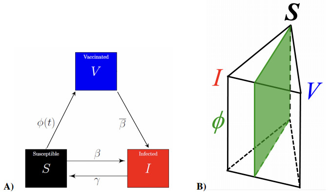
Vaccine hesitancy threatens to reverse the progress in tackling vaccine-preventable diseases. We used an $ SIS $ model with a game theory model for vaccination and parameters from the COVID-19 pandemic to study how vaccine hesitancy impacts epidemic dynamics. The system showed three asymptotic behaviors: total rejection of vaccinations, complete acceptance, and oscillations. With increasing fear of infection, stable endemic states become periodic oscillations. Our results suggest that managing fear of infection relative to vaccination is vital to successful mass vaccinations.
Citation: Anthony Morciglio, R. K. P. Zia, James M. Hyman, Yi Jiang. Understanding the oscillations of an epidemic due to vaccine hesitancy[J]. Mathematical Biosciences and Engineering, 2024, 21(8): 6829-6846. doi: 10.3934/mbe.2024299
Vaccine hesitancy threatens to reverse the progress in tackling vaccine-preventable diseases. We used an $ SIS $ model with a game theory model for vaccination and parameters from the COVID-19 pandemic to study how vaccine hesitancy impacts epidemic dynamics. The system showed three asymptotic behaviors: total rejection of vaccinations, complete acceptance, and oscillations. With increasing fear of infection, stable endemic states become periodic oscillations. Our results suggest that managing fear of infection relative to vaccination is vital to successful mass vaccinations.

| [1] | WHO, Ten Threats to Global Health in 2019. Available from: https://www.who.int/news-room/spotlight/ten-threats-to-global-health-in-2019. |
| [2] | Department of Health and Human Services, COVID-19 Vaccine Distribution: the Process. Available from: https://www.hhs.gov/coronavirus/covid-19-vaccines/index.html. |
| [3] |
W. Daniel, M. Nivet, J. Warner, D. K. Podolsky, Early evidence of the effect of SARS-CoV-2 vaccine at one medical center, N. Engl. J. Med., 384 (2021), 1962–1963. https://doi.org/10.1056/NEJMc2102153 doi: 10.1056/NEJMc2102153

|
| [4] | Centers for Disease Control and Prevention, COVID Data Tracker. Available from: https://covid.cdc.gov/covid-data-tracker/#datatracker-home. |
| [5] | Johns Hopkins Coronavirus Resource Center, Impact of Opening and Closing Decisions by State: A Look at How Social Distancing Measures May Have Inffuenced Trends in COVID-19 Cases and Death. Available from: https://coronavirus.jhu.edu/data/state-timeline. |
| [6] |
J. V. Lazarus, S. C. Ratzan, A. Palayew, L. O. Gostin, H. J. Larson, K. Rabin, et al., A global survey of potential acceptance of a COVID-19 vaccine, Nat. Med., 27 (2021), 225–228. https://doi.org/10.1038/s41591-020-1124-9 doi: 10.1038/s41591-020-1124-9
|
| [7] |
C. J. L. Murray, P. Piot, The potential future of the COVID-19 pandemic: Will SARS-CoV-2 become a recurrent seasonal infection?, JAMA, 325 (2021), 1249–1250. https://doi.org/10.1001/jama.2021.2828 doi: 10.1001/jama.2021.2828
|
| [8] |
J. McAteer, I. Yildirim, A. Chahroudi, The VACCINES Act: Deciphering vaccine hesitancy in the time of COVID-19, Clin. Infect. Dis., 71 (2020), 703–705. https://doi.org/10.1093/cid/ciaa433 doi: 10.1093/cid/ciaa433
|
| [9] |
A. A. Dror, N. Eisenbach, S. Taiber, N. G. Morozov, M. Mizrachi, A. Zigron, et al., Vaccine hesitancy: the next challenge in the ffght against COVID-19, Eur. J. Epidemiol., 35 (2020), 775–779. https://doi.org/10.1007/s10654-020-00671-y doi: 10.1007/s10654-020-00671-y
|
| [10] |
K. O. Kwok, K. K. Li, W. I. Wei, A. Tang, S. Y. S. Wong, S. S. Lee, Inffuenza vaccine uptake, COVID-19 vaccination intention and vaccine hesitancy among nurses: A survey, Int. J. Nurs. Stud., 114 (2021), 103854. https://doi.org/10.1007/s10654-020-00671-y doi: 10.1007/s10654-020-00671-y
|
| [11] |
R. Goodwin, M. Ben-Ezra, M. Takahashi, L. A. N. Luu, K. Borsfay, M. Kovács, et al., Psychological factors underpinning vaccine willingness in Israel, Japan and Hungary, Sci. Rep., 12 (2022), 439. https://doi.org/10.1038/s41598-021-03986-2 doi: 10.1038/s41598-021-03986-2
|
| [12] |
J. V. Lazarus, S. C. Ratzan, A. Palayew, L. O. Gostin, H. J. Larson, K. Rabin, et al., A global survey of potential acceptance of a COVID-19 vaccine, Nat. Med., 27 (2021), 225–228. https://doi.org/10.1038/s41591-020-1124-9 doi: 10.1038/s41591-020-1124-9
|
| [13] |
E. Robinson, A. Jones, I. Lesser, M. Daly, International estimates of intended uptake and refusal of COVID-19 vaccines: A rapid systematic review and meta-analysis of large nationally representative samples, Vaccine, 39 (2021), 2024–2034. https://doi.org/10.1038/s41591-020-1124-9 doi: 10.1038/s41591-020-1124-9
|
| [14] |
D. Freeman, B. Loe, A. Chadwick, C. Vaccari, F. Waite, L. Rosebrock, et al., COVID-19 vaccine hesitancy in the UK: the oxford coronavirus explanations, attitudes, and narratives survey (oceans) II, Psychol. Med., 52 (2022), 3127–3141. https://doi.org/10.1017/S0033291720005188 doi: 10.1017/S0033291720005188
|
| [15] |
C. Ghaznavi, D. Yoneoka, T. Kawashima, A. Eguchi, M. Murakami, S. Gilmour, et al., Factors associated with reversals of COVID-19 vaccination willingness: Results from two longitudinal, national surveys in Japan 2021–2022, Lancet Reg. Health–West. Paciffc, 27 (2022), 1–13. https://doi.org/10.1016/j.lanwpc.2022.100540 doi: 10.1016/j.lanwpc.2022.100540
|
| [16] |
M. Walkowiak, J. Domaradzki, D. Walkowiak, Are we facing a tsunami of vaccine hesitancy or outdated pandemic policy in times of omicron? analyzing changes of COVID-19 vaccination trends in Poland, Vaccines, 11 (2022), 1065. https://doi.org/10.3390/vaccines11061065 doi: 10.3390/vaccines11061065
|
| [17] |
J. Stoler, C. A. Klofstad, A. M. Enders, J. E. Uscinski, Sociopolitical and psychological correlates of COVID-19 vaccine hesitancy in the United States during summer 2021, Social Sci. Med., 306 (2022), 115112. https://doi.org/10.1016/j.socscimed.2022.115112 doi: 10.1016/j.socscimed.2022.115112
|
| [18] |
A. M. Enders, J. Uscinski, C. Klofstad, J. Stoler, On the relationship between conspiracy theory beliefs, misinformation, and vaccine hesitancy, PLoS One, 17 (2022), e0276082. https://doi.org/10.1371/journal.pone.0276082 doi: 10.1371/journal.pone.0276082
|
| [19] |
J. Uscinski, A. M. Enders, C. Klofstad, J. Stoler, Cause and effect: On the antecedents and consequences of conspiracy theory beliefs, Curr. Opin. Psychol., 47 (2022), 101364. https://doi.org/10.1016/j.copsyc.2022.101364 doi: 10.1016/j.copsyc.2022.101364
|
| [20] |
J. Murphy, F. Vallières, R. P. Bentall, M. Shevlin, O. McBride, T. K. Hartman, et al., Psychological characteristics associated with COVID-19 vaccine hesitancy and resistance in Ireland and the United Kingdom, Nat. Commun., 12 (2021), 29. https://doi.org/10.1038/s41467-020-20226-9 doi: 10.1038/s41467-020-20226-9
|
| [21] |
S. Hummert, K. Bohl, D. Basanta, A. Deutsch, S. Werner, G. Theissen, et al., Evolutionary game theory: cells as players, Mol. Biosyst., 10 (2014), 3044–3065. https://doi.org/10.1039/C3MB70602H doi: 10.1039/C3MB70602H
|
| [22] |
T. L. Vincent, J. S. Brown, Stability in an evolutionary game, Theor. Popul. Biol., 26 (1984), 408–427. https://doi.org/10.1039/C3MB70602H doi: 10.1039/C3MB70602H
|
| [23] | J. Hofbauer, K. Sigmund, Evolutionary game dynamics, Bull. Am. Math. Soc., 40 (2003), 479–519. https://doi.org/10.1090/S0273-0979-03-00988-1 |
| [24] | C. T. Bauch, D. J. D. Earn, Vaccination and the theory of games, in Proceedings of the National Academy of Sciences of the United States of America, 101 (2004), 13391–13394. https://doi.org/10.1073/pnas.0403823101 |
| [25] |
B. Rahman, E. Sadraddin, A. Porreca, The basic reproduction number of SARS-CoV-2 in wuhan is about to die out, how about the rest of the world, Rev. Med. Virol., 30 (2020), e2111. https://doi.org/10.1002/rmv.2111 doi: 10.1002/rmv.2111
|
| [26] |
M. A. Billah, M. M. Miah, M. N. Khan, Reproductive number of coronavirus: A systematic review and meta-analysis based on global level evidence, PLoS One, 15 (2020), e0242128. https://doi.org/10.1371/journal.pone.0242128 doi: 10.1371/journal.pone.0242128
|
| [27] |
H. Rossman, S. Shilo, T. Meir, M. Gorffne, U. Shalit, E. Segal, COVID-19 dynamics after a national immunization program in Israel, Nat. Med., 27 (2021), 1055–1061. https://doi.org/10.1038/s41591-021-01337-2 doi: 10.1038/s41591-021-01337-2
|
| [28] |
M. Voysey, S. A. C. Clemens, S. A. Madhi, L. Y. Weckx, P. M. Folegatti, P. K. Aley, et al., Single-dose administration and the inffuence of the timing of the booster dose on immunogenicity and efffcacy of ChAdOx1 nCoV-19 (AZD1222) vaccine: a pooled analysis of four randomised trials, Lancet, 397 (2021), 881–891. https://doi.org/10.1016/S0140-6736(21)00432-3 doi: 10.1016/S0140-6736(21)00432-3
|
| [29] | C. Luo, C. Morris, J. Sachithanandham, A. Amadi, D. Gaston, M. Li, et al., Infection with the SARS-CoV-2 delta variant is associated with higher infectious virus loads compared to the alpha variant in both unvaccinated and vaccinated individuals, medRxiv, 2021. https://doi.org/10.1101/2021.08.15.21262077 |
| [30] |
M. Lipsitch, SARS-CoV-2 breakthrough infections in vaccinated individuals: measurement, causes and impact, Nat. Rev. Immunol., 22 (2022), 57–65. https://doi.org/10.1038/s41577-021-00662-4 doi: 10.1038/s41577-021-00662-4
|
| [31] |
B. A. Cohn, P. M. Cirillo, C. C. Murphy, N. Y. Krigbaum, A. W. Wallace, SARS-CoV-2 vaccine protection and deaths among us veterans during 2021, Science, 375 (2022), 331–336. https://doi.org/10.1126/science.abm0620 doi: 10.1126/science.abm0620
|
| [32] |
S. T. Tan, A. T. Kwan, I. Rodríguez-Barraquer, B. J. Singer, H. J. Park, J. A. Lewnard, et al., Infectiousness of SARS-CoV-2 breakthrough infections and reinfections during the Omicron wave, Nat. Med., 29 (2023), 358–365. https://doi.org/10.1038/s41591-022-02138-x doi: 10.1038/s41591-022-02138-x
|
| [33] |
F. Guerra, S. Bolotin, G. Lim, J. Heffernan, S. Deeks, Y. Li, et al., The basic reproduction number (R0) of measles: a systematic review, Lancet Infect. Dis., 17 (2017), e420. https://doi.org/10.1016/S1473-3099(17)30307-9 doi: 10.1016/S1473-3099(17)30307-9
|
| [34] |
Y. Liu, J. Rocklöv, The effective reproductive number of the Omicron variant of SARS-CoV-2 is several times relative to Delta, J. Travel Med., 29 (2022), taac037. https://doi.org/10.1093/jtm/taac037 doi: 10.1093/jtm/taac037
|
| [35] | T. Randall, COVID Still Killing Americans Faster Than Guns, Cars and Flu Combined. Available from: https://www.bloomberg.com/news/articles/2021-07-16/how-many-COVID-deaths-still-more-than-guns-car-crashes-and-flu?leadSource = uverify%20wall. |
| [36] | University of Cambridge, How Have COVID-19 Fatalities Compared with Other Causes of Death. Available from: https://wintoncentre.maths.cam.ac.uk/coronavirus/how-have-COVID-19-fatalities-comparedother-causes-death/. |
| [37] |
K. M. Jia, W. P. Hanage, M. Lipsitch, A. G. Johnson, A. B. Amin, A. R. Ali, et al., Estimated preventable COVID-19-associated deaths due to non-vaccination in the United States, Eur. J. Epidemiol., 38 (2023), 1125–1128. https://doi.org/10.1007/s10654-023-01006-3 doi: 10.1007/s10654-023-01006-3
|
| [38] |
K. Y. Ng, M. M. Gui, COVID-19: Development of a robust mathematical model and simulation package with consideration for ageing population and time delay for control action and resusceptibility, Physica D, 411 (2020), 132599. https://doi.org/10.1016/j.physd.2020.132599 doi: 10.1016/j.physd.2020.132599
|
| [39] |
M. Angeli, G. Neofotistos, M. Mattheakis, E. Kaxiras, Modeling the effect of the vaccination campaign on the COVID-19 pandemic, Chaos, Solitons Fractals, 154 (2022), 111621. https://doi.org/10.1016/j.chaos.2021.111621 doi: 10.1016/j.chaos.2021.111621
|
| [40] |
T. Tsuruyama, Nonlinear model of infection wavy oscillation of COVID-19 in Japan based on diffusion kinetics, Sci. Rep., 12 (2022), 19177. https://doi.org/10.1038/s41598-022-23633-8 doi: 10.1038/s41598-022-23633-8
|
| [41] |
N. J. Stroud, Media use and political predispositions: Revisiting the concept of selective exposure, Polit. Behav., 30 (2008), 341–366. https://doi.org/10.1007/s11109-007-9050-9 doi: 10.1007/s11109-007-9050-9
|
| [42] |
N. J. Stroud, Polarization and partisan selective exposure, J. Commun., 60 (2010), 566–576. https://doi.org/10.1111/j.1460-2466.2010.01497.x doi: 10.1111/j.1460-2466.2010.01497.x
|
| [43] | N. J. Stroud, E. Thorson, D. Young, Making sense of information and judging its credibility, in Understanding and Addressing the Disinformation Ecosystem, (2017), 45–50. |


Figures(8) / Tables(2)

Anthony Morciglio, R. K. P. Zia, James M. Hyman, Yi Jiang. Understanding the oscillations of an epidemic due to vaccine hesitancy[J]. Mathematical Biosciences and Engineering, 2024, 21(8): 6829-6846. doi: 10.3934/mbe.2024299


 DownLoad: