
Citation: Olasimbo Fayombo. Everyday adaptations to flooding at the micro-levels of low-income communities and macro levels of authorities in the megacity of Lagos, Nigeria[J]. Urban Resilience and Sustainability, 2024, 2(2): 151-184. doi: 10.3934/urs.2024008
[1] | Chen Yue, Mingquan Ye, Peipei Wang, Daobin Huang, Xiaojie Lu . SRV-GAN: A generative adversarial network for segmenting retinal vessels. Mathematical Biosciences and Engineering, 2022, 19(10): 9948-9965. doi: 10.3934/mbe.2022464 |
[2] | Rafsanjany Kushol, Md. Hasanul Kabir, M. Abdullah-Al-Wadud, Md Saiful Islam . Retinal blood vessel segmentation from fundus image using an efficient multiscale directional representation technique Bendlets. Mathematical Biosciences and Engineering, 2020, 17(6): 7751-7771. doi: 10.3934/mbe.2020394 |
[3] | Yifan Zhang, Zhi Zhang, Shaohu Peng, Dongyuan Li, Hongxin Xiao, Chao Tang, Runqing Miao, Lingxi Peng . A rotation invariant template matching algorithm based on Sub-NCC. Mathematical Biosciences and Engineering, 2022, 19(9): 9505-9519. doi: 10.3934/mbe.2022442 |
[4] | Shenghan Li, Linlin Ye . Multi-level thresholding image segmentation for rubber tree secant using improved Otsu's method and snake optimizer. Mathematical Biosciences and Engineering, 2023, 20(6): 9645-9669. doi: 10.3934/mbe.2023423 |
[5] | Jiali Tang, Yan Wang, Chenrong Huang, Huangxiaolie Liu, Najla Al-Nabhan . Image edge detection based on singular value feature vector and gradient operator. Mathematical Biosciences and Engineering, 2020, 17(4): 3721-3735. doi: 10.3934/mbe.2020209 |
[6] | G. Prethija, Jeevaa Katiravan . EAMR-Net: A multiscale effective spatial and cross-channel attention network for retinal vessel segmentation. Mathematical Biosciences and Engineering, 2024, 21(3): 4742-4761. doi: 10.3934/mbe.2024208 |
[7] | Amsa Shabbir, Aqsa Rasheed, Huma Shehraz, Aliya Saleem, Bushra Zafar, Muhammad Sajid, Nouman Ali, Saadat Hanif Dar, Tehmina Shehryar . Detection of glaucoma using retinal fundus images: A comprehensive review. Mathematical Biosciences and Engineering, 2021, 18(3): 2033-2076. doi: 10.3934/mbe.2021106 |
[8] | Jinke Wang, Lubiao Zhou, Zhongzheng Yuan, Haiying Wang, Changfa Shi . MIC-Net: multi-scale integrated context network for automatic retinal vessel segmentation in fundus image. Mathematical Biosciences and Engineering, 2023, 20(4): 6912-6931. doi: 10.3934/mbe.2023298 |
[9] | Shudong Wang, Yuliang Lu, Xuehu Yan, Longlong Li, Yongqiang Yu . AMBTC-based visual secret sharing with different meaningful shadows. Mathematical Biosciences and Engineering, 2021, 18(5): 5236-5251. doi: 10.3934/mbe.2021266 |
[10] | Yu Li, Meilong Zhu, Guangmin Sun, Jiayang Chen, Xiaorong Zhu, Jinkui Yang . Weakly supervised training for eye fundus lesion segmentation in patients with diabetic retinopathy. Mathematical Biosciences and Engineering, 2022, 19(5): 5293-5311. doi: 10.3934/mbe.2022248 |
Retinal vascular network is a tree-like structure that includes arteries, arterioles, capillaries, veins and venules. It is useful to find the other normal features of retina such as macula or fovea or optic disk or for the automatic identification of pathological elements like hemorrhage, micro aneurysms, exudates or lesions [1]. As vascular diseases present a challenging health problem for society, so an efficient vascular segmentation algorithm is needed for understanding and analysis of vascular diseases in a better way. Segmentation of blood vessels using manual method and semi-automatic method is tedious and time consuming task because high skills and training is required in both these methods. Moreover, these segmentation techniques are susceptible to errors. With the use of fully automatic segmentation techniques, problems of manual segmentation and semi-automatic segmentation can be overcome. These automatic techniques are helpful in the advancement of computer-aided diagnostic systems which are used for identification of various ophthalmic disorders. Segmentation of vessels in an accurate manner is a tedious job because of the less variations in the contrast between vasculature and surrounding tissue, presence of noise in the retina image; variation in the vessel width, shape, branching angle and brightness of image and presence of lesions, exudates, hemorrhage and other pathologies.
Although various segmentation techniques have been used [2,3,4] for segmentation of different diseases and anatomical structures of the body but the main goal of this paper is to present the methodology used for extraction of vessels from fundus image. Modified Pixel level snake (PLS) technique has been used for extraction of vessels. PLS is an iterative technique, in which internal and external forces are used for evolution of pixels of contour. Various segmentation approaches can be used for extraction of blood vessels, which includes unsupervised approach [5,6,7,8], supervised approach [9,10,11,12,13,14,15,16], tracking approach [17,18,19], deformable models approach [20,21,22,23,24,25,26], filtering approach [27] and morphological approach [28,31].
Stall et al. [29] proposed a method for extraction of ridges of image from the color retinal fundus image. Soares et al. [30] presented a technique in which enhancement of retinal fundus image is performed using gabor filter and classification is performed using Bayesian classifier. Martinez et al. [32] proposed a method based on multiscale feature extraction approach for segmentation of vasculature map from red-free and fluorescein retinal fundus images. You et al. [33] presented a scheme based on the radial projection and semi-supervised method, for the extraction of retinal vasculature map. Alonso-Montes et al. [40] proposed a method based on PLS. In this, PLS has been used and tested in single instruction multiple data (SIMD) parallel processor array, for segmentation of retinal vasculature map. Time of execution and accuracy has also been analyzed. Perfetti et al. [41] proposed Cellular neural network (CNN) technique for extraction of vessels. Normally, in PLS, external potential is computed using edge based techniques. In our proposed methodology, BTH transformation is used for the computation of external potential, which results in improved accuracy of the extracted vasculature map.
Contribution of the proposed approach is as follows:
● Bimodal masking is applied for the extraction of the mask of the fundus image.
● Global thresholding is used for segmentation of vasculature map of fundus image.
● MPLS based on BTH transformation has been proposed for evolution of map in four cardinal directions.
The remaining paper is structured as follows. Section 2 described the materials used for proposed work. Section 3 described the methodology used for extraction of the vasculature map of the fundus image. Section 4 represented the results and discussions and section 5 represented the conclusion of the work.
For analysis purpose, the color fundus image of the retina has been taken from the DRIVE (Digital Retinal Images for Vessels Extraction) database [42]. This database contains 40 images, out of which 20 are test images and 20 are training images. Out of 40 images, 7 images are pathological images and 33 are normal images. Images are produced at 45° field of view (FOV), using Canon CR5 nonmydriatic 3CCd camera. Size of each image in this database is 565 × 584 pixels.
After implementation of the algorithm on the DRIVE dataset, simulation is also performed on 20 images (700 × 605 pixels each) of the STARE (Structured Analysis of Retina) database [43].
Pixel based classification is used for extraction of vasculature map from the fundus image. Pixel classification is done on the basis of whether the pixel belongs to the vessel or surrounding tissue. So, four different possible events are possible which include pixel classifications and pixel misclassifications. True positive (TP) and true negative (TN) are the two pixel classifications and false positive (FP), and false negative (FN) are the two pixel misclassifications which are used for evaluation of various performance metrics. An event is classified as TP if a vessel pixel is correctly identified as vessel and TN if the non-vessel pixel or pixel in the surrounding tissue is correctly identified as a non-vessel pixel. An event is said to be FN if the predicted pixel represents a non-vessel pixel but actually it was a vessel pixel. An event is said to be FP if the predicted pixel represents vessel pixel but actually it was a non-vessel pixel. The important performance metrics which can be derived from the above events are sensitivity, specificity, and accuracy.
SN metrics represents the ability of a segmentation method to detect the vessel pixels. SN is defined as the ratio of TP to the sum of TP and FN. Range of sensitivity is between 0 and 1. More SN means the algorithm is able to identify vessel pixels correctly. SN measure is expressed by Eq (1).
SN=TP(TP+FN) | (1) |
SP metrics represents the ability of a segmentation algorithm to detect background or non-vessel pixels. SP is also defined as the ratio of TN to the sum of TN and FP. Range of specificity is also between 0 and 1. More SP means the algorithm is able to identify non-vessel pixels correctly. SP measure is expressed by Eq (2).
SP=TN(TN+FP) | (2) |
Acc is evaluated by taking the ratio of total number of true events which is the sum of TP and TN, to the total population which is the total number of pixels actually present in the image. The formula for accuracy is expressed by Eq (3).
Acc=TP+TNTP+TN+FP+FN | (3) |
Proposed methodology for automated extraction of vasculature map of fundus image is presented in Figure 1. The main components of the pre-processing are: RGB to gray conversion, generation of mask using bimodal masking and contrast enhancement using CLAHE (Contrast Limited Adaptive Histogram Equalization).
Initially RGB fundus image (1_test of DRIVE database) is read and converted to gray scale image for segmentation of vessels. Conversion of RGB to gray image also reduces the time required for processing of the image. Different weights for R, G & B components are selected for conversion purpose. RGB to gray conversion is performed using the formula represented by Eq (4) [44].
G=0.2989∗r+0.5870∗ g+0.1140∗ b | (4) |
Where r, g and b symbolize the red, green, and blue channels of the fundus image respectively and G is the gray image produced after conversion. The green channel is the channel which gives the maximum information of the fundus image, so the weight of the green channel is chosen larger as compared to other channels. RGB image and its corresponding gray-scale image is represented by Figure 2(a), (b) respectively.
Vasculature map of retinal fundus image is used for detection of diseases and monitoring of diseases. After applying certain image processing techniques on fundus images, the speed of analyzing these images can be increased. Since analyses require more time and computational effort, operations should be focused only on the object pixels. For getting the object pixels, first the binary mask is generated and then multiplied with the original image so as to get the accurate image required for segmentation.Flow chart for the generation of mask using bimodal masking is shown in Figure 2(c). Mask is generated from the gray image, obtained after RGB to gray conversion. Initially histogram of image is generated as shown in Figure 2(d) and then dominant peaks and valleys are identified according to the histogram [45]. Then the second valley is selected as threshold level for the conversion of gray image into binary image. Binary image is produced after thresholding is termed as final mask, shown in Figure 2(e). Figure 2(f) represents the mask of image, produced after simple thresholding techniques. So, it can be easily analyzed that the mask produced after bimodal masking is accurate as compared to simple thresholding technique.
CLAHE operation is performed for enhancement of contrast of an image. CLAHE works on small areas in the image rather than the entire image. These small regions are termed as 'tiles'. Enhancement of contrast has been performed tile wise. After that all neighboring tiles are combined using bilinear interpolation method. In this paper, two level enhancements have been done using CLAHE technique. It means CLAHE has been applied two times for getting the proper enhanced image. Size of tiles used for CLAHE is [8 8] and the number of bins is 128. Enhanced image produced after applying CLAHE technique is shown in Figure 3(a).
The main component of the pre-processing is global thresholding used for extraction of initial contour.
Enhanced image produced using CLAHE is further used to produce the segmented image. For generation of segmented image, initially adaptive segmentation is required because gray values along vessels in retina vasculature are non-uniform. Input of adaptive segmentation is preprocessed image (enhanced image) and output is segmented image. Figure 3(b) represents the block diagram of adaptive segmentation. Average filter having size 9 is applied on preprocessed image to produce averaged image as shown in Figure 3(c). After that, a subtracted image is produced by taking the difference between the averaged image and the preprocessed image. Then a global thresholding technique is applied on the subtracted image for computation of threshold level of image. Global thresholding technique (Algorithm 1) is stated as follows:
Algorithm 1: Global thresholding technique. |
1. Choose an initial random threshold T for segmentation. This threshold is called the global threshold. 2. Using threshold T, segment the fundus image. Two groups of pixels are produced: (i) All pixels having value more than T, belong to group G1. (ii) All pixels having value less than or equal to T, belong to group G2. 3. Evaluate the average intensities m1 and m2 of both the groups G1 and G2 respectively. 4. Again compute the threshold using T = (1/2)(m1 + m2). 5. Repeat steps 2-4 until the successive iterations threshold difference is smaller than the already defined value. 6. Segment the image by taking T as threshold value. |
Using this threshold, the subtracted image is converted to the binary image, which is called as the segmented image as represented by Figure 3(d). This segmented image will be used to find the initial contour which is defined implicitly as the region boundary. After that morphological operation, closing is applied on the segmented image by taking disk shaped structuring element (SE) having size 1. Then small areas having pixel size less than 35 are removed from the closed image. The image produced is called the initial contour of the image shown in Figure 3(e).
Next task is to remove the border from the contour image because the retinal vasculature map does not include the outer border as shown in the initial contour image represented by Figure 3(e). So, the border is removed from the initial contour image using the mask produced using bimodal masking. To perform this operation, the initial contour image is subtracted from the complement of the mask. If after subtraction, some pixels contain values greater than 0, then value 1 is assigned to those pixels and if some pixels contain values less than zero, then 0 is assigned to those pixels. So after subtraction and assigning values to the subtracted image, a contour image without border is produced. After that morphological operation (dilation) using disk shape SE having size 1 is applied on the image. The image shown in Figure 3(f) is further used for evolution using MPLS.
The main components of the post processing are evolution of contour using modified PLS and removal of noise.
In a PLS algorithm the evolution of contour is performed by pixel-by-pixel shifting of the contour, towards a position where the potential is minimum. Figure 4 shows the flowchart of PLS algorithm. In this algorithm, contour pixels evolve iteratively according to the potential field. This potential field comprises of three potentials named as internal, external and balloon potential and the weights of these potentials are adjusted according to the application. The main components of a PLS algorithm is contour evolution. Topological Transformations module is also used to handle merging and splitting of contours. This module is basically used to avoid collisions between contours.
(1) External potential computation
In existing methods, external potential is calculated using edge based techniques like sobel and canny edge detection. But in this paper, MPLS is proposed in which external potential of image is calculated by using BTH transformation method because the external potential produced using BTH method contains more information about the vasculature map resulting in higher accuracy. Using this external potential, the total potential of the image is computed which evolves the contour in an efficient way as compared to previous existing methods. Flow chart for computation of external potential for modified PLS is shown in Figure 5(a). Here, BTH transformation is applied on the green channel of the retinal fundus image (as shown by Figure 5(b)) by taking three different structuring elements.
The BTH transform is the transformation which is evaluated by subtracting the input image from the closing of the input image. The BTH transform of image (f) is given by Eq (5).
Tb(I)=I⊙b−I | (5) |
Here, I is the input image; b represents the SE and ⊙ represents the closing operation.
Output Tb(I) represents the BTH transformed image.
Three different disk shaped structuring elements having size 2, 7, 11 are used for closing operation in computation of external potential. Then the sum of all three BTH transformed images is taken to produce the external potential image as represented by Figure 5(c). For evolution of contour towards minimum potential, complement of external potential is taken. Complement of external potential image (Pe) is represented by Figure 5(d).
This is the potential which guides the contour of the image towards edges of the vasculature map. If the image is static, then external potential is computed once. Applications like real time computer vision, in which moving images are there, external potential is computed for each frame of the image. Evolution of PLS will be done by external potential which is stronger in areas close to the edges.
(2) Internal potential computation
This potential is useful in maintaining the smooth shape of the contour. During the evolution of PLS, all vessel discontinuities are avoided using internal potential. Internal potential is computed from the initial contour. Flow chart for computation of internal potential of the image is shown in Figure 6(a). In this, initially a binary contour edge image is produced from the initial contour image shown in Figure 5(e) using the expression: C = IC and not (ICN and ICS and ICW and ICE). Here IC represents the initial contour of the image, ICN represents IC(x, y - 1), i.e., active region pixels in NORTH direction from the current pixel IC(x, y).Similarly ICE, ICW and ICS represents IC(x, y+1), IC(x -1, y), IC(x+1, y), i.e., active region pixels in East, West and South directions from the current pixel IC(x, y) respectively. Figure 6(b) represents the edge image produced from the initial contour image. Diffusion of image has been performed on edge image of initial contour by anisotropic diffusion method taking lambda = 0.25; and no. of iterations = 20. Anisotropic diffusion of contour image is performed to obtain an internal potential field. Anisotropic diffusion, also called Perona-Malik diffusion, is a technique used to reduce noise present in the image without removing important parts of the image content.
Anisotropic diffusion is defined by Eq (6).
∂I∂t=div(c(x,y,t)∇I)=∇c.∇I+c(x,y,t)ΔI | (6) |
Where Δ denotes the laplacian, ∇ denotes the gradient, div is the divergence operator and c(x, y, t) is the diffusion coefficient. Two functions for diffusion coefficient are proposed by Perona and Malik which are representedby Eqs 7(a) and 7(b).
c(‖∇I‖)=e−(‖∇I‖K)2 | (7a) |
And
c(‖∇I‖)=11+(‖∇I‖K)2 | (7b) |
Constant K is used to control the sensitivity to edges. Here the value of K is chosen as 40. The diffused image as shown in Figure 6(c) is multiplied with weight having value 0.1 to get an internal potential image. After that, the complement of the internal potential image (Pi) has been taken for contour evolution in the proper direction. Figure 6(d), (e) represent the weighted internal potential image and complemented image respectively.
(3) Balloon potential computation
When external potential is too weak, then it's not possible for external potential to guide the contour in all directions. In that case, there is one potential which produces forces, to guide the contour towards object pixels. Initially PLS is controlled by balloon potential because initially contour is far from vessel edges. To get balloon potential image, initial contour is multiplied with weight having value 0.1. Flowchart for computation of balloon potential is shown in Figure 7(a). Figure 7(b), (c) represents weighted balloon potential and complement of balloon potential image (Pb) respectively.
(4) Guiding force extraction module
Potential field is computed as the weighted sum of external, internal and balloon potential as represented by equation 8. All internal and external forces are produced through the potential field that guides the evolution of contour towards minimum energy level.
PT=Pe+Pi+Pb | (8) |
Here PT represents the total potential field of an image, Pe represents the external potential of image, Pi represents the internal potential image and Pb represents the balloon potential of image. Figure 7(d) represents the potential field image produced after the addition of all potential images.
(5) Directional contour evolution with topological transformation and collision detection module
Evolution of directional contour is the most important part of PLS technique. It is performed in four prime directions: NORTH, EAST, WEST and SOUTH (NEWS). After iteration each pixel of contour is moved towards a position, where it can acquire minimum potential.
The expansion of contour may result in merging and splitting of contours. But in segmentation of retinal vasculature, it's required to prevent the collision between the contours. For preventing the collision, a collision detection module has been used. When contour expands in each direction, the two vessels may combine with each other. So, this expansion of contour is done in such a way that there should be no danger of collision. Figure 8(a) represents the different cases for dangers of collisions. Considering the danger of collision point in mind, expression for expansion in NORTH, SOUTH, EAST and WEST direction is computed below.
Expansion in north direction:
Pixel wise expansion of initial contour has been performed in the north direction based on potential of image. Expression for expansion in NORTH direction is given by Condition 1.
If (not D) and ICS and (PT < PT S), then IC becomes equal to 1. Cond.(1)
Here D = R or RE or RW and R = (not IC) and ICN.
Here, PT represents the total potential field, PTS represents potential field in south direction, R represents the active/background pixel pairs in the vertical direction, D represents the danger of collision which is determined by taking logic 'OR' of the current pixel of R with its east (RE) and west (RW) neighbor.
Expansion of the initial contour in the north direction is represented by taking a matrix of 10:10 elements. Figures 8(b), (c) represents the initial contour of 100 pixels and its expanded version in north direction respectively. Observe the pixel values and potential of initial contour highlighted with red box in Figure 8(d), (e) respectively. If the pixel has value 0 and its potential is less than potential in its south direction, then value 1 is assigned to that pixel as represented in Figure 8(f).
Similarly, expressions in other directions can be computed by considering the danger of collision.
Expression in south direction is given by Cond.(2)
If (not D) and ICN and (PT < PTN) then IC becomes equal to 1. Cond.(2)
Here D = R or RE or RW and R = (not IC) and ICS.
Expression in east direction is given by Cond.(3)
If (not D) and ICW and (PT < PTW) then IC becomes equal to 1. Cond.(3)
Here D = R or RN or RS and R = (not IC) and ICE.
Expression in west direction is given by Cond.(4)
If (not D) and ICE and (PT < PTE) then IC becomes equal to 1. Cond.(4)
Here D = R or RN or RS and R = (not IC) and ICW.
Images produced after expansion in N, S, E, W directions are represented by Figure 9(a)-(d).
(6) Inversion
Image produced after expansion in all directions is inverted to ensure contour evolution towards minimum potential. Inversion of the active region produces a new contour shifted by one pixel. So, the inverted image is not simply calculated by (not IC) but using the following expression.
Inv = (not IC) or c. Here c = IC and not (ICN and ICS and ICW and ICE). Inverted image is represented by Figure 10(a). After inversion, evolution of contour image is again performed in all directions. So, expansion and contraction of active and background regions is performed in each iteration. Also steady direction of forces which are inflating and deflating in nature, can be maintained by inverting balloon potential after each iteration. Figure 10(b)-(e) represents contour expansion in all directions in the second iteration respectively.
In the last stage, small objects (extracted from retinal vasculature obtained after MPLS evolution) having pixels less than 30 are removed. Noise which is present outside the border has been removed by multiplying the final vasculature map with the complement of mask. After that morphological closing with SE disk having size 1 is applied on the image. This is the final vasculature map as shown by Figure 11(a), which can be further used for identification of various diseases.
Various performance metrics such as SN, SP and Acc have been computed by using extracted vasculature map and ground truth map. Acc of proposed algorithm is better is due to extraction of accurate binary mask of fundus image; better enhancement of image and evolution of vasculature map using MPLS technique in all four cardinal directions. Figure 11(a), (b) represents extracted map and ground truth image of original retinal fundus image.
The algorithm can be applied on all images of the DRIVE database. Figure 12 represents the results of the three normal images of the DRIVE database and their extracted vasculature map respectively.
Table 1 represents comparative analysis of SN, SP and Acc metrics for DRIVE database. For analysis purpose, the proposed method results are compared with the results obtained by Staal [29] et al., Soares [30] et al., Mendonc-a [31] et al., Martinez-Perez [32] et al., You [33] et al., Fraz [34] et al., Ravichandran et al. [35], Zhao et al. [36], Yin et al. [37], Frucci [38] et al. and Zhang [39] et al., Adapa [46], Ma [47]. It has been observed that for MPLS, average SN comes out to be better than existing methodologies except [47] and SP comes out to be better than existing methodologies except [38], because there is a trade-off between SN and SP of image. Acc of proposed methodology is better than Acc of all existing methodologies.
Method | Year | SN | SP | Acc |
Staal [29] | 2004 | 0.7194 | 0.9773 | 0.9442 |
Soares [30] | 2006 | 0.7230 | 0.9762 | 0.9446 |
Mendonc-a [31] | 2006 | 0.7344 | 0.9764 | 0.9452 |
Martinez-Perez [32] | 2007 | 0.7246 | 0.9655 | 0.9344 |
You [33] | 2011 | 0.7410 | 0.9751 | 0.9434 |
Fraz [34] | 2012 | 0.7406 | 0.9807 | 0.9480 |
Ravichandran [35] | 2014 | 0.7259 | 0.9799 | 0.9574 |
Zhao [36] | 2014 | 0.7354 | 0.9789 | 0.9477 |
Yin [37] | 2015 | 0.7246 | 0.9790 | 0.9403 |
Frucci [38] | 2016 | 0.670 | 0.986 | 0.959 |
Zhang [39] | 2017 | 0.7861 | 0.9712 | 0.9466 |
Adapa [46] | 2019 | 0.6994 | 0.9811 | 0.945 |
Ma [47] | 2020 | 0.7875 | 0.9813 | 0.9566 |
Proposed Method | 2021 | 0.76959 | 0.9834 | 0.9630 |
This algorithm has been tested on all test images and pathological images of the DRIVE database. Figure 13 represents the results of the two pathological images of the DRIVE database and their extracted vasculature map respectively. Table 2 represents SN, SP and Acc results for 5 pathological images of the DRIVE database. It has been observed that the average SN, SP and Acc for pathological images is 70.80%, 96.40% and 94.41% respectively. Simulation has also been performed on 20 images of the STARE dataset. Table 3 shows the comparative analysis of average values of SN, SP and Acc for different images of STARE dataset and it has been observed that proposed technique has high Acc even for the STARE dataset also which proves the robust nature of proposed algorithm.
Image | SN | SP | Acc |
1 | 0.6769 | 0.9941 | 0.9664 |
2 | 0.7617 | 0.9646 | 0.9519 |
3 | 0.7483 | 0.9220 | 0.9083 |
4 | 0.7012 | 0.9868 | 0.9702 |
5 | 0.6522 | 0.9523 | 0.9239 |
Average | 70.80 | 96.40 | 94.41 |
Method | Year | SN | SP | Acc |
Soares et al. [30] | 2006 | 0.7181 | 0.9765 | 0.9500 |
Fraz et al. [34] | 2012 | 0.7262 | 0.9764 | 0.9511 |
Azzopardi et al. [7] | 2015 | 0.7716 | 0.9701 | 0.9497 |
Li et al. [16] | 2015 | 0.7726 | 0.9844 | 0.9628 |
Roychowdhury et al. [8] | 2016 | 0.7720 | 0.9730 | 0.9510 |
Li et al. [48] | 2017 | 0.7843 | 0.9837 | 0.9690 |
WA-Net [47] | 2020 | 0.7740 | 0.9871 | 0.9645 |
Proposed Work | 2021 | 0.7930 | 0.9895 | 0.9745 |
Accurate segmentation of the vasculature map of the fundus image plays a crucial role in the diagnostic procedure of various retinal disorders. In the proposed work, initially the binary mask of fundus image is generated using bimodal masking technique and vasculature map is extracted using global thresholding technique. MPLS technique has been used for evolution of contour in all directions to extract the vasculature map in accurate manner. Simulated results demonstrate that the proposed technique can extract vasculature maps of normal images as well as pathological images accurately. Since the methodology used for extraction of vessels is unsupervised, no training is required. Vessel connectivity has also been done without any danger of collision. Proposed algorithm is an efficient technique because it is used for extraction of vasculature maps from normal as well as pathological images. Further extracted vasculature maps can be used to find the features of retina such as macula or fovea or optic disk or for the automatic identification of pathological elements like hemorrhage, microaneurysms, exudates or lesions accurately. Also the quantitative and objective assessment of arteriovenous nicking can be performed in future.
We would like to show our gratitude to Dr. Mausumi Acharyya, AdvenioTechnoSys, India, for sharing their pearls of wisdom with us during this research. The authors would like to thank people who provide the public databases used in this work.
The authors declare no conflict of interest in this paper.
[1] |
Satterthwaite D (2013) The political underpinnings of cities' accumulated resilience to climate change. Environ Urban 25: 381–391. https://doi.org/10.1177/0956247813500902 doi: 10.1177/0956247813500902
![]() |
[2] | IPCC (Intergovernmental Panel on Climate Change) (2014) Fifth assessment report AR5—Urban areas, Chapter 8, IPCC WGII. Available from: https://www.ipcc.ch/assessment-report/ar5/. |
[3] |
Dow K, Berkhout F, Preston BL, et al. (2013) Limits to adaptation. Nat Clim Chang 3: 305–307. https://doi.org/10.1038/nclimate1847 doi: 10.1038/nclimate1847
![]() |
[4] |
Hardoy J, Pandiella G (2009) Urban poverty and vulnerability to climate change in Latin America. Environ Urban 21: 203–224. https://doi.org/10.1177/0956247809103019 doi: 10.1177/0956247809103019
![]() |
[5] | Eriksen SEH, Klien RJT, Ulsrud K, et al. (2007) Climate change adaptation and poverty reduction: Key interactions and critical measures. Report prepared for the Norwegian Agency for Development Cooperation (NORAD). GECHS Rep 1–44. Available from: https://citeseerx.ist.psu.edu/document?repid=rep1&type=pdf&doi=29621d9367d85986362aa32fe06998e5b7049f27. |
[6] |
Khan MR, Roberts JT (2013) Adaptation and international climate policy. Wiley Interdiscip Rev Clim Change 4: 171–189. https://doi.org/10.1002/wcc.212 doi: 10.1002/wcc.212
![]() |
[7] |
Tol RSJ, Downing TE, Kuik OJ, et al. (2004) Distributional aspects of climate change impacts. Global Environ Change 14: 259–272. https://doi.org/10.1016/j.gloenvcha.2004.04.007 doi: 10.1016/j.gloenvcha.2004.04.007
![]() |
[8] | Satterthwaite D, Huq S, Reid H, et al. (2009) Adapting to climate change in urban areas: The possibilities and constraints in low and middle-income nations, In: Adapting Cities to Climate Change, Earthscan, UK: Routledge, 3–47. |
[9] |
Ajibade I, McBean G, Bezner-Kerr R (2013) Urban flooding in Lagos, Nigeria: Patterns of vulnerability and resilience among women. Global Environ Change 23: 1714–1725. https://doi.org/10.1016/j.gloenvcha.2013.08.009 doi: 10.1016/j.gloenvcha.2013.08.009
![]() |
[10] |
Manuel-Navarrete D, Pelling M, Redclift M (2011) Critical adaptation to hurricanes in the Mexican Caribbean: Development visions, governance structures, and coping strategies. Global Environ Change 21: 249–258. https://doi.org/10.1016/j.gloenvcha.2010.09.009 doi: 10.1016/j.gloenvcha.2010.09.009
![]() |
[11] | Moser CON, Satterthwaite D (2008) Towards pro-poor adaptation to climate change in the urban centres of low-and middle-income countries, In: Human Settlement Development Series: Climate Change and Cities Discussion Paper 3, London: International Institute for Environment and Development (ⅡED). |
[12] | Adelekan IO, Simpson NP, Totin E, et al. (2022) IPCC sixth assessment report (AR6)—Impacts, adaptation and vulnerability: Regional factsheet Africa. Available from: https://www.ipcc.ch/report/ar6/wg2/about/factsheets/. |
[13] |
Huq S, Kovats S, Reid H, et al. (2007) Reducing risks to cities from disasters and climate change. Environ Urban 19: 7–15. https://doi.org/10.1177/0956247807078058 doi: 10.1177/0956247807078058
![]() |
[14] | IPCC (Intergovernmental Panel on Climate Change) (2007) Fourth assessment report AR4—Summary for policy makers. Available from: https://www.ipcc.ch/report/ar4/wg1/summary-for-policymakers/. |
[15] |
Chen AS, Djordjević S, Leandro J, et al. (2010) An analysis of the combined consequences of pluvial and fluvial flooding. Water Sci Technol 62: 1491–1498. https://doi.org/10.2166/wst.2010.486 doi: 10.2166/wst.2010.486
![]() |
[16] | UN-Habitat (2014) The State of African Cities, 2014: Re-imagining Sustainable Urban Transitions. Kenya: UN-Habitat. |
[17] |
De Sherbinin A, Schiller A, Pulsipher A (2007) The vulnerability of global cities to climate hazards. Environ Urban 19: 39–64. https://doi.org/10.1177/0956247807076725 doi: 10.1177/0956247807076725
![]() |
[18] | BNRCC (2012) Towards a Lagos State Climate Change Adaptation Strategy (LAS-CCAS). Available from: http://csdevnet.org/wp-content/uploads/Towards-aLagos-Adaptation-Strategy.pdf. |
[19] | Sunday OA, Ajewole AI (2006) Implications of the changing pattern of landcover of the Lagos Coastal Area of Nigeria. Am-Eurasian J Sci Res 1: 31–37. |
[20] | Lagos State Government-Ministry of the Environment (LASG-MoE) (2012) Lagos State Climate Change Policy 2012–2014. |
[21] | Ogunleye M, Alo B (2011) State of the environment report-Lagos, 2010. Ministry of the Environment, Lagos State/Beachland Resources Limited. |
[22] |
Elias P, Omojola A (2015) Case study: the challenges of climate change for Lagos, Nigeria. Curr Opin Environ Sustain 13: 74–78. https://doi.org/10.1016/j.cosust.2015.02.008 doi: 10.1016/j.cosust.2015.02.008
![]() |
[23] |
Komolafe AA, Adegboyega SAA, Anifowose AYB, et al. (2014) Air pollution and climate change in Lagos, Nigeria: needs for proactive approaches to risk management and adaptation. Am J Environ Sci 10: 412. https://doi.org/10.3844/ajessp.2014.412.423 doi: 10.3844/ajessp.2014.412.423
![]() |
[24] | Oshaniwa T, Chikwendu C (2013) Climate change mapping in some constituencies in Lagos State. Policy Advocacy Project Partnership on Climate Change (PAPPCC). |
[25] | UNIDO (United Nations Industrial Development Organization) (2010) Climate change scenario and coastal risk analysis study of Lagos State of Nigeria. |
[26] | Heinemann ASS, Moser C, Norton A, et al. (2010) Pro-poor adaptation to climate change in urban centers: Case studies of vulnerability and resilience in Kenya and Nicaragua. World Bank. Available from: http://documents.worldbank.org/curated/en/2010/06/14829757/pro-poor-adaptation-climate-change-urban-centers-case-studies-vulnerability-resilience-kenya-nicaragua. |
[27] |
Douglas I, Alam K, Maghenda M, et al. (2008) Unjust waters: climate change, flooding, and the urban poor in Africa. Environ Urban 20: 187–205. https://doi.org/10.1177/0956247808089156 doi: 10.1177/0956247808089156
![]() |
[28] |
Reddy BS, Assenza GB (2009) The great climate debate. Energy Policy 37: 2997–3008. https://doi.org/10.1016/j.enpol.2009.03.064 doi: 10.1016/j.enpol.2009.03.064
![]() |
[29] |
Alam M, Rabbani MDG (2007) Vulnerabilities and responses to climate change for Dhaka. Environ Urban 19: 81–97. https://doi.org/10.1177/0956247807076911 doi: 10.1177/0956247807076911
![]() |
[30] |
Awuor CB, Orindi VA, Ochieng Adwera A (2008) Climate change and coastal cities: the case of Mombasa, Kenya. Environ Urban 20: 231–242. https://doi.org/10.1177/0956247808089158 doi: 10.1177/0956247808089158
![]() |
[31] |
Castán Broto V, Oballa B, Junior P (2013) Governing climate change for a just city: Challenges and lessons from Maputo, Mozambique. Local Environ 18: 678–704. https://doi.org/10.1080/13549839.2013.801573 doi: 10.1080/13549839.2013.801573
![]() |
[32] |
Abam TKS, Ofoegbu CO, Osadebe CC, et al. (2000) Impact of hydrology on the Port-Harcourt–Patani-Warri Road. Environ Geol 40: 153–162. https://doi.org/10.1007/s002540000106 doi: 10.1007/s002540000106
![]() |
[33] | NEMA (National Emergency Management Agency) (2013) Flood: NEMA urges governments stakeholders collaboration. |
[34] | Oladunjoye M (2011) Flooding: Lagos gives relief materials to victims. Available from: http://allafrica.com/stories/201109080792.htmlaccessed23/11/2023. |
[35] |
Adelekan IO (2010) Vulnerability of poor urban coastal communities to flooding in Lagos, Nigeria. Environ Urban 22: 433–451. https://doi.org/10.1177/0956247810380141 doi: 10.1177/0956247810380141
![]() |
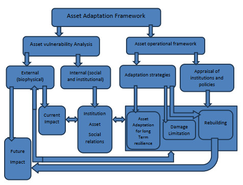
[36] | Moser C (2011) A conceptual and operational framework for pro-poor asset adaptation to urban climate change, In: Cities and Climate Change, 2011: 225–254. |
[37] |
Thomas DSG, Twyman C (2005) Equity and justice in climate change adaptation amongst natural-resource-dependent societies. Global Environ Change 15: 115–124. https://doi.org/10.1016/j.gloenvcha.2004.10.001 doi: 10.1016/j.gloenvcha.2004.10.001
![]() |
[38] |
Hoornweg D, Sugar L, Trejos Gomez CL (2011) Cities and greenhouse gas emissions: moving forward. Environ Urban 23: 207–227. https://doi.org/10.1177/0956247810392270 doi: 10.1177/0956247810392270
![]() |
[39] |
Kates RW, Travis WR, Wilbanks TJ (2012) Transformational adaptation when incremental adaptations to climate change are insufficient. Proc Natl Acad Sci 109: 7156–7161. https://doi.org/10.1073/pnas.1115521109 doi: 10.1073/pnas.1115521109
![]() |
[40] |
Kates RW (2000) Cautionary tales: adaptation and the global poor. Clim Change 45: 5–17. https://doi.org/10.1023/A:1005672413880 doi: 10.1023/A:1005672413880
![]() |
[41] | Lemos MC, Agrawal A, Eakin H, et al. (2013) Building adaptive capacity to climate change in less developed countries, In: Asrar, G., Hurrell, J. Author, Climate Science for Serving Society, Dordrecht: Springer, 437–457. https://doi.org/10.1007/978-94-007-6692-1-16 |
[42] |
While A, Whitehead M (2013) Cities, urbanisation, and climate change. Urban Stud 50: 1325–1331. https://doi.org/10.1177/0042098013480963 doi: 10.1177/0042098013480963
![]() |
[43] |
Barrett S (2012) The necessity of a multi-scalar analysis of climate justice. Prog Hum Geogr 37: 215–233. https://doi.org/10.1177/0309132512448270 doi: 10.1177/0309132512448270
![]() |
[44] |
Kelly PM, Adger WN (2000) Theory and practice in assessing vulnerability to climate change and facilitating adaptation. Clim Change 47: 325–352. https://doi.org/10.1023/A:1005627828199 doi: 10.1023/A:1005627828199
![]() |
[45] |
Adger WN, Huq S, Brown K, et al. (2003) Adaptation to climate change in the developing world. Prog Dev Stud 3: 179–195. https://doi.org/10.1191/1464993403ps060oa doi: 10.1191/1464993403ps060oa
![]() |
[46] | Huq S, Reid H (2004) Mainstreaming adaptation in development. IDS Bull 35: 15–21. Available from: https://opendocs.ids.ac.uk/opendocs/bitstream/handle/20.500.12413/8546/IDSB-35-3-10.1111-j.1759-5436.2004.tb00129.x.pdf?sequence=1. |
[47] | Prowse M, Scott L (2008) Assets and adaptation: an emerging debate. IDS Bull 39: 42–52. Available from: https://opendocs.ids.ac.uk/opendocs/bitstream/handle/20.500.12413/8197/IDSB-39-4-10.1111-j.1759-5436.2008.tb00475.x.pdf?sequence=1. |
[48] | Moser CON, Satterthwaite D (2011) Towards a pro poor adaptation in the urban centres of low and middle-income countries. Available from: https://hummedia.manchester.ac.uk/institutes/mui/gurg/working-papers/GURC-wp1.pdf. |
[49] |
Tanner T, Mitchell T (2008) Entrenchment or enhancement: could climate change adaptation help reduce chronic poverty?. Chron Poverty Res Cent Work Pap. doi: https://dx.doi.org/10.2139/ssrn.1629175. doi: 10.2139/ssrn.1629175
![]() |
[50] |
Moser CON (1998) The asset vulnerability framework: reassessing urban poverty reduction strategies. World Dev 26: 1–19. https://doi.org/10.1016/S0305-750X(97)10015-8 doi: 10.1016/S0305-750X(97)10015-8
![]() |
[51] |
Moser CON (2017) Gender transformation in a new global urban agenda: challenges for Habitat Ⅲ and beyond. Environ Urban 29: 221–236. https://doi.org/10.1177/0956247816662573 doi: 10.1177/0956247816662573
![]() |
[52] |
Ribot JC, Peluso NL (2003) A theory of access. Rural Sociol 68: 153–181. https://doi.org/10.1111/j.1549-0831.2003.tb00133.x doi: 10.1111/j.1549-0831.2003.tb00133.x
![]() |
[53] |
Mitlin D (2003) Addressing urban poverty through strengthening assets. Habitat Int 27: 393–406. https://doi.org/10.1016/S0197-3975(02)00066-8 doi: 10.1016/S0197-3975(02)00066-8
![]() |
[54] |
Rakodi C (2006) Relationships of power and place: the social construction of African cities. Geoforum 37: 312–317. https://doi.org/10.1016/j.geoforum.2005.10.001 doi: 10.1016/j.geoforum.2005.10.001
![]() |
[55] |
Bebbington A (1999) Capitals and capabilities: a framework for analysing peasant viability, rural livelihoods, and poverty. World Dev 27: 2021–2044. https://doi.org/10.1016/S0305-750X(99)00104-7 doi: 10.1016/S0305-750X(99)00104-7
![]() |
[56] |
Parnell S, Simon D, Vogel C (2007) Global Environmental Change: Conceptualising the growing challenge for cities in poor countries. Area 39: 357–369. https://doi.org/10.1111/j.1475-4762.2007.00760.x doi: 10.1111/j.1475-4762.2007.00760.x
![]() |
[57] | UN-Habitat (2011) Global report on human settlements 2011: cities and climate change. Kenya: United Nations Human Settlements Programme. Available from: https://unhabitat.org/global-report-on-human-settlements-2011-cities-and-climate-change. |
[58] |
Friend R, Moench M (2013) What is the purpose of urban climate resilience? Implications for addressing poverty and vulnerability. Urban Clim 6: 98–113. https://doi.org/10.1016/j.uclim.2013.09.002 doi: 10.1016/j.uclim.2013.09.002
![]() |
[59] |
Bulkeley H, Tuts R (2013) Understanding urban vulnerability, adaptation, and resilience in the context of climate change. Local Environ 18: 646–662. https://doi.org/10.1080/13549839.2013.788479 doi: 10.1080/13549839.2013.788479
![]() |
[60] |
Moser C, Stein A (2011) Implementing urban participatory climate change adaptation appraisals: a methodological guideline. Environ Urban 23: 463–485. https://doi.org/10.1177/0956247811418739 doi: 10.1177/0956247811418739
![]() |
[61] |
Füssel HM, Klein RJ (2006) Climate change vulnerability assessments: an evolution of conceptual thinking. Clim Change 75: 301–329. https://doi.org/10.1007/s10584-006-0329-3 doi: 10.1007/s10584-006-0329-3
![]() |
[62] |
Luers AL (2005) The surface of vulnerability: An analytical framework for examining environmental change. Global Environ Change 15: 214–223. https://doi.org/10.1016/j.gloenvcha.2005.04.003 doi: 10.1016/j.gloenvcha.2005.04.003
![]() |
[63] | Yamin F, Rahman A, Huq S (2005) Vulnerability, adaptation and climate disasters: A conceptual overview. IDS Bull 36: 1–14. |
[64] |
Cannon T, Müller-Mahn D (2010) Vulnerability, resilience, and development discourses in context of climate change. Nat Hazard 55: 621–635. https://doi.org/10.1007/s11069-010-9499-4 doi: 10.1007/s11069-010-9499-4
![]() |
[65] | Field CB, Barros V, Stocker T, et al. (2012) Managing the Risks of Extreme Events and Disasters to Advance Climate Change Adaptation: Special Report of the Intergovernmental Panel on Climate Change, Cambridge: Cambridge University Press, 30: 7575–7613. https://doi.org/10.1017/CBO9781139177245 |
[66] | Pelling M (2011) Adaptation to Climate Change from Resilience to Transformation. London: Taylor and Francis Books. https://doi.org/10.4324/9780203889046 |
[67] |
Leichenko R (2011) Climate change and urban resilience. Curr Opin Environ Sustain 3: 164–168. https://doi.org/10.1016/j.cosust.2010.12.014 doi: 10.1016/j.cosust.2010.12.014
![]() |
[68] | Mitchell T, Harris K (2012) Resilience: A risk management approach. ODI Backgr Note 2012: 1–7. |
[69] |
Nelson DR, Adger WN, Brown K (2007) Adaptation to environmental change: contributions of a resilience framework. Annu Rev Environ Resour 32: 395–419. https://doi.org/10.1146/annurev.energy.32.051807.090348 doi: 10.1146/annurev.energy.32.051807.090348
![]() |
[70] |
Harris LM, Chu EK, Ziervogel G (2018) Negotiated resilience. Resilience 6: 196–214. https://doi.org/10.1080/21693293.2017.1353196 doi: 10.1080/21693293.2017.1353196
![]() |
[71] |
Béné C, Newsham A, Davies M, et al. (2014) Resilience, poverty, and development. J Int Dev 26: 598–623. https://doi.org/10.1002/jid.2992 doi: 10.1002/jid.2992
![]() |
[72] |
Pelling M, Dill K (2010) Disaster politics: tipping points for change in the adaptation of sociopolitical regimes. Prog Hum Geogr 34: 21–37. https://doi.org/10.1177/0309132509105004 doi: 10.1177/0309132509105004
![]() |
[73] |
Adger WN, Quinn T, Lorenzoni I, et al. (2013) Changing social contracts in climate-change adaptation. Nat Clim Chang 3: 330–333. https://doi.org/10.1038/nclimate1751 doi: 10.1038/nclimate1751
![]() |
[74] |
Eriksen SH, Nightingale AJ, Eakin H (2015) Reframing adaptation: the political nature of climate change adaptation. Glob Environ Change 35: 523–533. https://doi.org/10.1016/j.gloenvcha.2015.09.014 doi: 10.1016/j.gloenvcha.2015.09.014
![]() |
[75] |
Manuel‐Navarrete D (2010) Power, realism, and the ideal of human emancipation in a climate of change. Wiley Interdiscip Rev Clim Change 1: 781–785. https://doi.org/10.1002/wcc.87 doi: 10.1002/wcc.87
![]() |
[76] |
Revi A, Satterthwaite D, Aragón-Durand F, et al. (2014) Towards transformative adaptation in cities: the IPCC's Fifth Assessment. Environ Urban 26: 11–28. https://doi.org/10.1177/0956247814523539 doi: 10.1177/0956247814523539
![]() |
[77] |
Ribot J (2011) Vulnerability before adaptation: Toward transformative climate action. Glob Environ Change 21: 1160–1162. http://doi.org/10.1016/j.gloenvcha.2011.07.008 doi: 10.1016/j.gloenvcha.2011.07.008
![]() |
[78] | Strengers Y (2010) Conceptualising everyday practices: composition, reproduction, and change. Carbon Neutral Communities Centre for Design, RMIT University. |
[79] |
Heinrichs D, Krellenberg K, Fragkias M (2013) Urban responses to climate change: theories and governance practice in cities of the global south. Int J Urban Reg Res 37: 1865–1878. https://doi.org/10.1111/1468-2427.12031 doi: 10.1111/1468-2427.12031
![]() |
[80] |
O'Brien K (2012) Global environmental change Ⅱ: from adaptation to deliberate transformation. Prog Hum Geogr 36: 667–676. https://doi.org/10.1177/0309132511425767 doi: 10.1177/0309132511425767
![]() |
[81] |
Woolcock M, Narayan D (2000) Social capital: Implications for development theory, research, and policy. World Bank Res Obs 15: 225–249. https://doi.org/10.1093/wbro/15.2.225 doi: 10.1093/wbro/15.2.225
![]() |
[82] |
Adger WN (2003) Social capital, collective action, and adaptation to climate change. Econ Geogr 79: 387–404. https://doi.org/10.1007/978-3-531-92258-4-19 doi: 10.1007/978-3-531-92258-4-19
![]() |
[83] |
Pelling M, High C (2005) Understanding adaptation: what can social capital offer assessments of adaptive capacity? Glob Environ Change 15: 308–319. https://doi.org/10.1016/j.gloenvcha.2005.02.001 doi: 10.1016/j.gloenvcha.2005.02.001
![]() |
[84] |
Bebbington A, Perreault T (1999) Social capital, development, and access to resources in highland Ecuador. Econ Geogr 75: 395–418. https://doi.org/10.1111/j.1944-8287.1999.tb00127.x doi: 10.1111/j.1944-8287.1999.tb00127.x
![]() |
[85] |
Luthans F, Luthans KW, Luthans BC (2004) Positive psychological capital: Beyond human and social capital. Bus Horiz 47: 45–50. https://doi.org/10.1016/j.bushor.2003.11.007 doi: 10.1016/j.bushor.2003.11.007
![]() |
[86] | Becker GS (1994) Human capital revisited, In: Human Capital: A Theoretical and Empirical Analysis with Special Reference to Education, the University of Chicago Press. |
[87] | Moser C (2008) Assets and livelihoods: a framework for asset-based social policy, In: Dani, A.A., Moser, C. Author, Assets, Livelihoods, and Social Policy, Washington DC: World Bank, 43–82. |
[88] |
Bassett TJ, Fogelman C (2013) Déjà vu or something new? The adaptation concept in the climate change literature. Geoforum 48: 42–53. https://doi.org/10.1016/j.geoforum.2013.04.010 doi: 10.1016/j.geoforum.2013.04.010
![]() |
[89] | Creswell JW (2014) A Concise Introduction to Mixed Methods Research. Sage Publications. |
[90] | Bryman A (2012) Social Research Methods. Oxford: Oxford University Press. |
[91] | Desai V, Potter RB (2006) Doing Development Research. London: Sage. https://doi.org/10.4135/9781849208925 |
[92] |
Olorunnimbe RO, Oni SI, Ege E, et al. (2022) Analysis of effects of prolonged travel delay on public bus operators' profit margin in metropolitan Lagos, Nigeria. J Sustain Dev Transp Logist 7: 112–126. https://doi.org/10.14254/jsdtl.2022.7-1.10 doi: 10.14254/jsdtl.2022.7-1.10
![]() |
[93] | Lagos State Urban Renewal Authority (LASURA) (2013) Slum identification Handbook: A compendium of Nine (9) Major Slums in Lagos Metropolis. Lagos State Government Ministry of Physical Planning and Urban Development. Document obtained from LASURA office, Lagos Nigeria. |
[94] |
Sanchez-Rodriguez R (2009) Learning to adapt to climate change in urban areas. A review of recent contributions. Curr Opin Environ Sustain 1: 201–206. https://doi.org/10.1016/j.cosust.2009.10.005 doi: 10.1016/j.cosust.2009.10.005
![]() |
[95] | Valentine G (2013) Tell me about … using interviews as a research methodology, In: Fowerdew, R., Martin, D. Author, Methods in Human Geograph, London: Routledge, 110–127. |
[96] |
Valentine G (1999) Being seen and heard? The ethical complexities of working with children and young people at home and at school. Ethics Place Environ 2: 141–155. https://doi.org/10.1080/1366879X.1999.11644243 doi: 10.1080/1366879X.1999.11644243
![]() |
[97] |
Berrang-Ford L, Ford JD, Paterson J (2011) Are we adapting to climate change? Glob Environ Change 21: 25–33. https://doi.org/10.1016/j.gloenvcha.2010.09.012 doi: 10.1016/j.gloenvcha.2010.09.012
![]() |
[98] | Twum KO, Abubakari M (2019) Cities and floods: A pragmatic insight into the determinants of households' coping strategies to floods in informal Accra, Ghana. Jàmbá: J Disaster Risk Stud 11: 1–14. https://hdl.handle.net/10520/EJC-13b8ce4b99 |
[99] | Sakijege T, Lupala J, Sheuya S (2012) Flooding, flood risks and coping strategies in urban informal residential areas: The case of Keko Machungwa, Dar es Salaam, Tanzania. Jàmbá: J Disaster Risk Stud 4: 1–10. https://hdl.handle.net/10520/EJC125636 |
[100] |
Chatterjee M (2010) Slum dwellers response to flooding events in the megacities of India. Mitigation Adapt Strategies Global Change 15: 337–353. https://doi.org/10.1007/s11027-010-9221-6 doi: 10.1007/s11027-010-9221-6
![]() |
[101] |
Wamsler C, Brink E (2014) Moving beyond short-term coping and adaptation. Environ Urban 26: 86–111. https://doi.org/10.1177/0956247813516061 doi: 10.1177/0956247813516061
![]() |
[102] |
Haque AN, Dodman D, Hossain MM (2014) Individual, communal, and institutional responses to climate change by low-income households in Khulna, Bangladesh. Environ Urban 26: 112–129. https://doi.org/10.1177/0956247813518681 doi: 10.1177/0956247813518681
![]() |
[103] | Jooste BS, Dokken JV, Van Niekerk D, et al. (2018) Challenges to belief systems in the context of climate change adaptation. Jàmbá: J Disaster Risk Stud 10: 1–10. https://hdl.handle.net/10520/EJC-110b8aa4c0 |
[104] |
Gaillard JC, Texier P (2010) Religions, natural hazards, and disasters: An introduction. Religion 40: 81–84. https://doi.org/10.1016/j.religion.2009.12.001 doi: 10.1016/j.religion.2009.12.001
![]() |
[105] | Schuman S, Dokken JV, Van Niekerk D, et al. (2018) Religious beliefs and climate change adaptation: A study of three rural South African communities. Jàmbá: J Disaster Risk Stud 10: 1–12. https://hdl.handle.net/10520/EJC-122cafb0c5 |
[106] |
Mitchell JT (2003) Prayer in disaster: Case study of Christian clergy. Nat Hazards Rev 4: 20–26. https://doi.org/10.1061/(ASCE)1527-6988(2003)4:1(20) doi: 10.1061/(ASCE)1527-6988(2003)4:1(20)
![]() |
[107] | Sachdeva S (2016) Religious identity, beliefs, and views about climate change, In: Oxford Research Encyclopedia of Climate Science, Oxford University Press. https://doi.org/10.1093/acrefore/9780190228620.013.335 |
[108] |
Billig M (2006) Is my home my castle? Place attachment, risk perception, and religious faith. Environ Behav 38: 248–265. https://doi.org/10.1177/0013916505277608 doi: 10.1177/0013916505277608
![]() |
[109] |
Scannell L, Gifford R (2013) Personally relevant climate change: The role of place attachment and local versus global message framing in engagement. Environ Behav 45: 60–85. https://doi.org/10.1177/0013916511421196 doi: 10.1177/0013916511421196
![]() |
[110] | Ribot JC, Chhatre A, Lankina T (2008) Introduction: institutional choice and recognition in the formation and consolidation of local democracy. Conserv Soc 6: 1–11. |
[111] | Omolara O (2022) An empirical analysis of the influence of values, worldview, and culture on the psychological processes in transformational adaptation. London J Res Humanit Soc Sci 22: 1–24. |
[112] | O'Brien K, Hayward B, Berkes F (2009) Rethinking social contracts: building resilience in a changing climate. Ecol Soc 14: 12. https://www.jstor.org/stable/26268331 |
[113] |
Shackleton S, Ziervogel G, Sallu S, et al. (2015) Why is socially‐just climate change adaptation in sub‐Saharan Africa so challenging? A review of barriers identified from empirical cases. Wiley Interdiscip Rev Clim Change 6: 321–344. https://doi.org/10.1002/wcc.335 doi: 10.1002/wcc.335
![]() |
[114] | Cornwall A (2002) Locating citizen participation. IDS Bull 33: i–x. Available from: https://opendocs.ids.ac.uk/opendocs/bitstream/handle/20.500.12413/8659/IDSB_33_2_10.1111-j.1759-5436.2002.tb00016.x.pdf?sequence=1accessed24/11/2023. |
[115] | Federal Ministry of Environment (2004) National erosion and flood control policy. Available from: https://searchworks.stanford.edu/view/7884006. |
[116] | Lagos State Government Ministry of the Environment (2012) Ministerial press briefing. LASG-Ministry of the Environmnet (MoE). |
[117] | Lagos State Government (2001) Environmental sanitation law 2000, supplement to the Lagos State of Nigeria official gazette extraordinary. Obtained from Agboyi Ketu Local Council Development Authority. |
[118] |
Oshodi L (2013) Flood management and governance structure in Lagos, Nigeria. Reg Mag 292: 22–24. https://doi.org/10.1080/13673882.2013.10815622 doi: 10.1080/13673882.2013.10815622
![]() |
[119] |
Soneye A (2014) An overview of humanitarian relief supply chains for victims of perennial flood disasters in Lagos, Nigeria (2010–2012). J Humanit Logist Supply Chain Manag 4: 179–197. https://doi.org/10.1108/JHLSCM-01-2014-0004 doi: 10.1108/JHLSCM-01-2014-0004
![]() |
[120] |
Nkwunonwo UC, Whiteworth M, Bailey B (2015) Review article: a review and critical analysis of the efforts towards urban flood reduction in the Lagos region of Nigeria. Nat Hazard Earth Syst Sci Discuss 3: 667–676. https://doi.org/10.5194/nhess-16-349-2016 doi: 10.5194/nhess-16-349-2016
![]() |
[121] | Federal Ministry of Environment (2005) Technical guidelines on erosion and flood control and coastal zone management. Available from: https://environment.gov.ng/. |
[122] |
Fatti CE, Patel Z (2013) Perceptions and responses to urban flood risk: Implications for climate governance in the South. Appl Geogr 36: 13–22. https://doi.org/10.1016/j.apgeog.2012.06.011 doi: 10.1016/j.apgeog.2012.06.011
![]() |
[123] |
Adger WN, Dessai S, Goulden M, et al. (2009) Are there social limits to adaptation to climate change? Clim Change 93: 335–354. https://doi.org/10.1007/s10584-008-9520-z doi: 10.1007/s10584-008-9520-z
![]() |
[124] |
Harvatt J, Petts J, Chilvers J (2011) Understanding householder responses to natural hazards: flooding and sea‐level rise comparisons. J Risk Res 14: 63–83. https://doi.org/10.1080/13669877.2010.503935 doi: 10.1080/13669877.2010.503935
![]() |
[125] |
Graham S, Barnett J, Fincher R, et al. (2013) The social values at risk from sea-level rise. Environ Impact Assess Rev 41: 45–52. https://doi.org/10.1016/j.eiar.2013.02.002 doi: 10.1016/j.eiar.2013.02.002
![]() |
[126] |
Cheshire L (2015) 'Know your neighbours': disaster resilience and the normative practices of neighbouring in an urban context. Environ Plan A 47: 1081–1099. https://doi.org/10.1177/0308518X15592310 doi: 10.1177/0308518X15592310
![]() |
[127] |
Pelling M, O'Brien K, Matyas D (2015) Adaptation and transformation. Clim Change 133: 113–127. https://doi.org/10.1007/s10584-014-1303-0 doi: 10.1007/s10584-014-1303-0
![]() |
[128] | Painter J, Jeffrey A (2012) Political Geography: An Introduction to Space and Power. London: Sage. |
[129] |
Carmen E, Fazey I, Ross H, et al. (2022) Building community resilience in a context of climate change: The role of social capital. Ambio 51: 1371–1387. https://doi.org/10.1007/s13280-021-01678-9 doi: 10.1007/s13280-021-01678-9
![]() |
[130] |
Fazey I, Carmen E, Ross H, et al. (2021) Social dynamics of community resilience building in the face of climate change: The case of three Scottish communities. Sustain Sci 16: 1731–1747. https://doi.org/10.1007/s11625-021-00950-x doi: 10.1007/s11625-021-00950-x
![]() |
[131] | Olsson P, Gunderson LH, Carpenter SR, et al. (2006) Shooting the rapids: navigating transitions to adaptive governance of social-ecological systems. Ecol Soc 11. https://www.jstor.org/stable/26267806 |
[132] |
Leck H, Roberts D (2015) What lies beneath: understanding the invisible aspects of municipal climate change governance. Curr Opin Environ Sustain 13: 61–67. https://doi.org/10.1016/j.cosust.2015.02.004 doi: 10.1016/j.cosust.2015.02.004
![]() |
[133] |
Ellis E (2006) Citizenship and property rights: A new look at social contract theory. J Polit 68: 544–555. https://doi.org/10.1111/j.1468-2508.2006.00444.x doi: 10.1111/j.1468-2508.2006.00444.x
![]() |
[134] |
Mishra S, Mazumdar S, Suar D (2010) Place attachment and flood preparedness. J Environ Psychol 30: 187–197. https://doi.org/10.1016/j.jenvp.2009.11.005 doi: 10.1016/j.jenvp.2009.11.005
![]() |
[135] |
Adger WN, Barnett J, Brown K, et al. (2013) Cultural dimensions of climate change impacts and adaptation. Nat Clim Change 3: 112–117. https://doi.org/10.1038/nclimate1666 doi: 10.1038/nclimate1666
![]() |
[136] |
Geschiere P, Jackson S (2006) Autochthony and the crisis of citizenship: democratization, decentralization, and the politics of belonging. Afr Stud Rev 49: 1–8. https://doi.10.1353/arw.2006.0104 doi: 10.1353/arw.2006.0104
![]() |
[137] | Dunn KC (2009) 'Sons of the Soil' and Contemporary State Making: autochthony, uncertainty, and political violence in Africa, In: Third World Quarterly, London: Routledge, 30: 113–127. |
[138] |
Kraxberger B (2005) Strangers, indigenes, and settlers: contested geographies of citizenship in Nigeria. Space Polity 9: 9–27. https://doi.org/10.1080/13562570500078576 doi: 10.1080/13562570500078576
![]() |
[139] |
Adebanwi W (2009) Terror, territoriality and the struggle for indigeneity and citizenship in northern Nigeria. Citiz Stud 13: 349–363. https://doi.org/10.1080/13621020903011096 doi: 10.1080/13621020903011096
![]() |
[140] |
Cannon T (2008) Vulnerability, "innocent" disasters and the imperative of cultural understanding. Disaster Prev Manag 17: 350–357. https://doi.org/10.1108/09653560810887275 doi: 10.1108/09653560810887275
![]() |
[141] |
Shove E (2010) Beyond the ABC: Climate change policy and theories of social change. Environ Plan A 42: 1273–1285. https://doi.org/10.1068/a42282 doi: 10.1068/a42282
![]() |
[142] |
Kaika M (2017) 'Don't call me resilient again!' the New Urban Agenda as immunology… or… what happens when communities refuse to be vaccinated with 'smart cities' and indicators. Environ Urban 29: 89–102. https://doi.org/10.1177/0956247816684763 doi: 10.1177/0956247816684763
![]() |
[143] |
Pelling M (1998) Participation, social capital, and vulnerability to urban flooding in Guyana. J Int Dev 10: 469–486. https://doi.org/10.1002/(SICI)1099-1328(199806)10:4<469::AID-JID539>3.0.CO;2-4 doi: 10.1002/(SICI)1099-1328(199806)10:4<469::AID-JID539>3.0.CO;2-4
![]() |
[144] |
Fayombo OO (2021) Discursive constructions underlie and exacerbate the vulnerability of informal urban communities to the impacts of climate change. Clim Dev 13: 293–305. https://doi.org/10.1080/17565529.2020.1765133 doi: 10.1080/17565529.2020.1765133
![]() |
[145] |
Gasper R, Blohm A, Ruth M (2011) Social and economic impacts of climate change on the urban environment. Curr Opin Environ Sustain 3: 150–157. https://doi.org/10.1016/j.cosust.2010.12.009 doi: 10.1016/j.cosust.2010.12.009
![]() |
![]() |
![]() |
1. | Vatsala Anand, Sheifali Gupta, Deepika Koundal, Soumya Ranjan Nayak, Paolo Barsocchi, Akash Kumar Bhoi, Modified U-NET Architecture for Segmentation of Skin Lesion, 2022, 22, 1424-8220, 867, 10.3390/s22030867 | |
2. | Goldy Verma, 2024, Xception Model for Accurate Indian Rock Python Detection in Deep Learning, 979-8-3315-2963-5, 406, 10.1109/ICUIS64676.2024.10866422 |
Algorithm 1: Global thresholding technique. |
1. Choose an initial random threshold T for segmentation. This threshold is called the global threshold. 2. Using threshold T, segment the fundus image. Two groups of pixels are produced: (i) All pixels having value more than T, belong to group G1. (ii) All pixels having value less than or equal to T, belong to group G2. 3. Evaluate the average intensities m1 and m2 of both the groups G1 and G2 respectively. 4. Again compute the threshold using T = (1/2)(m1 + m2). 5. Repeat steps 2-4 until the successive iterations threshold difference is smaller than the already defined value. 6. Segment the image by taking T as threshold value. |
Method | Year | SN | SP | Acc |
Staal [29] | 2004 | 0.7194 | 0.9773 | 0.9442 |
Soares [30] | 2006 | 0.7230 | 0.9762 | 0.9446 |
Mendonc-a [31] | 2006 | 0.7344 | 0.9764 | 0.9452 |
Martinez-Perez [32] | 2007 | 0.7246 | 0.9655 | 0.9344 |
You [33] | 2011 | 0.7410 | 0.9751 | 0.9434 |
Fraz [34] | 2012 | 0.7406 | 0.9807 | 0.9480 |
Ravichandran [35] | 2014 | 0.7259 | 0.9799 | 0.9574 |
Zhao [36] | 2014 | 0.7354 | 0.9789 | 0.9477 |
Yin [37] | 2015 | 0.7246 | 0.9790 | 0.9403 |
Frucci [38] | 2016 | 0.670 | 0.986 | 0.959 |
Zhang [39] | 2017 | 0.7861 | 0.9712 | 0.9466 |
Adapa [46] | 2019 | 0.6994 | 0.9811 | 0.945 |
Ma [47] | 2020 | 0.7875 | 0.9813 | 0.9566 |
Proposed Method | 2021 | 0.76959 | 0.9834 | 0.9630 |
Image | SN | SP | Acc |
1 | 0.6769 | 0.9941 | 0.9664 |
2 | 0.7617 | 0.9646 | 0.9519 |
3 | 0.7483 | 0.9220 | 0.9083 |
4 | 0.7012 | 0.9868 | 0.9702 |
5 | 0.6522 | 0.9523 | 0.9239 |
Average | 70.80 | 96.40 | 94.41 |
Method | Year | SN | SP | Acc |
Soares et al. [30] | 2006 | 0.7181 | 0.9765 | 0.9500 |
Fraz et al. [34] | 2012 | 0.7262 | 0.9764 | 0.9511 |
Azzopardi et al. [7] | 2015 | 0.7716 | 0.9701 | 0.9497 |
Li et al. [16] | 2015 | 0.7726 | 0.9844 | 0.9628 |
Roychowdhury et al. [8] | 2016 | 0.7720 | 0.9730 | 0.9510 |
Li et al. [48] | 2017 | 0.7843 | 0.9837 | 0.9690 |
WA-Net [47] | 2020 | 0.7740 | 0.9871 | 0.9645 |
Proposed Work | 2021 | 0.7930 | 0.9895 | 0.9745 |