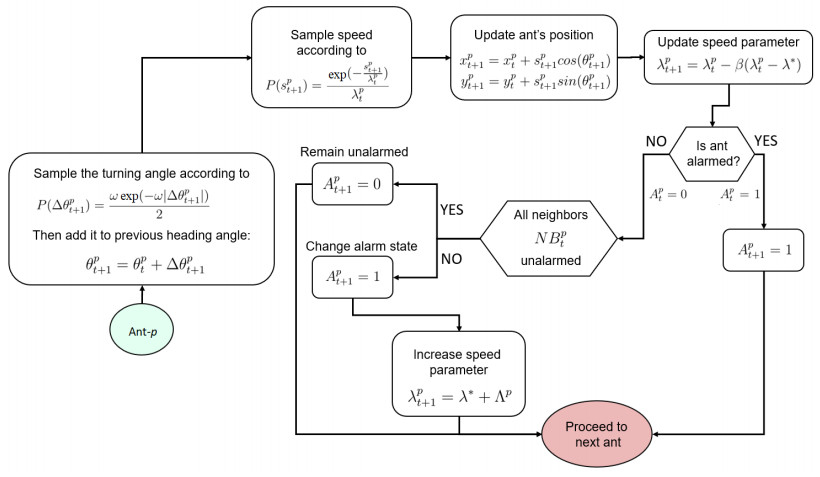
Ant colonies demonstrate a finely tuned alarm response to potential threats, offering a uniquely manageable empirical setting for exploring adaptive information diffusion within groups. To effectively address potential dangers, a social group must swiftly communicate the threat throughout the collective while conserving energy in the event that the threat is unfounded. Through a combination of modeling, simulation, and empirical observations of alarm spread and damping patterns, we identified the behavioral rules governing this adaptive response. Experimental trials involving alarmed ant workers (Pogonomyrmex californicus) released into a tranquil group of nestmates revealed a consistent pattern of rapid alarm propagation followed by a comparatively extended decay period [
Citation: Michael R. Lin, Xiaohui Guo, Asma Azizi, Jennifer H. Fewell, Fabio Milner. Mechanistic modeling of alarm signaling in seed-harvester ants[J]. Mathematical Biosciences and Engineering, 2024, 21(4): 5536-5555. doi: 10.3934/mbe.2024244
Ant colonies demonstrate a finely tuned alarm response to potential threats, offering a uniquely manageable empirical setting for exploring adaptive information diffusion within groups. To effectively address potential dangers, a social group must swiftly communicate the threat throughout the collective while conserving energy in the event that the threat is unfounded. Through a combination of modeling, simulation, and empirical observations of alarm spread and damping patterns, we identified the behavioral rules governing this adaptive response. Experimental trials involving alarmed ant workers (Pogonomyrmex californicus) released into a tranquil group of nestmates revealed a consistent pattern of rapid alarm propagation followed by a comparatively extended decay period [

| [1] |
X. Guo, M. R. Lin, A. Azizi, L. P. Saldyt, Y. Kang, T. P. Pavlic, et al., Decoding alarm signal propagation of seed-harvester ants using automated movement tracking and supervised machine learning, Proc. R. Soc. B, 289 (2022), 20212176. https://doi.org/10.1098/rspb.2021.2176 doi: 10.1098/rspb.2021.2176

|
| [2] |
O. Feinerman, A. Korman, Individual versus collective cognition in social insects, J. Exp. Biol., 220 (2017), 73–82. https://doi.org/10.1242/jeb.143891 doi: 10.1242/jeb.143891
|
| [3] |
B. Doerr, M. Fouz, T. Friedrich, Why rumors spread fast in social networks, Commun. ACM, 55 (2012), 70–75. https://doi.org/10.1145/2184319.2184338 doi: 10.1145/2184319.2184338
|
| [4] |
L. Bonnasse-Gahot, H. Berestycki, M. Depuiset, M. B. Gordon, S. Roché, N. Rodriguez, et al., Epidemiological modelling of the 2005 french riots: A spreading wave and the role of contagion, Sci. Rep., 8 (2018), 107. https://doi.org/10.1038/s41598-017-18093-4 doi: 10.1038/s41598-017-18093-4
|
| [5] |
D. A. Sprague, T. House, Evidence for complex contagion models of social contagion from observational data, PLoS One, 12 (2017), 1–12. https://doi.org/10.1371/journal.pone.0180802 doi: 10.1371/journal.pone.0180802
|
| [6] |
C. E. Coltart, B. Lindsey, I. Ghinai, A. M. Johnson, D. L. Heymann, The ebola outbreak, 2013–2016: Old lessons for new epidemics, Phil. Trans. R. Soc. B, 372 (2017), 20160297. https://doi.org/10.1098/rstb.2016.0297 doi: 10.1098/rstb.2016.0297
|
| [7] | B. Hölldobler, E. O. Wilson, The Ants, Harvard University Press, 1990. |
| [8] |
F. E. Regnier, E. O. Wilson, The alarm-defence system of the ant acanthomyops claviger, J. Insect Physiol., 14 (1968), 955–970. https://doi.org/10.1016/0022-1910(68)90006-1 doi: 10.1016/0022-1910(68)90006-1
|
| [9] |
W. H. Bossert, E. O. Wilson, The analysis of olfactory communication among animals, J. Theor. Biol., 5 (1963), 443–469. https://doi.org/10.1016/0022-5193(63)90089-4 doi: 10.1016/0022-5193(63)90089-4
|
| [10] |
E. Frehland, B. Kleutsch, H. Markl, Modelling a two-dimensional random alarm process, BioSystems, 18 (1985), 197–208. https://doi.org/10.1016/0303-2647(85)90071-1 doi: 10.1016/0303-2647(85)90071-1
|
| [11] |
D. J. McGurk, J. Frost, E. J. Eisenbraun, K. Vick, W. A. Drew, J. Young, Volatile compounds in ants: Identification of 4-methyl-3-heptanone from Pogonomyrmex ants, J. Insect Physiol., 12 (1966), 1435–1441. https://doi.org/10.1016/0022-1910(66)90157-0 doi: 10.1016/0022-1910(66)90157-0
|
| [12] |
J. B. Xavier, J. M. Monk, S. Poudel, C. J. Norsigian, A. V. Sastry, C. Liao, et al., Mathematical models to study the biology of pathogens and the infectious diseases they cause, Iscience, 25 (2022), 104079. https://doi.org/10.1016/j.isci.2022.104079 doi: 10.1016/j.isci.2022.104079
|
| [13] |
P. Törnberg, Echo chambers and viral misinformation: Modeling fake news as complex contagion, PLoS One, 13 (2018), 1–21. https://doi.org/10.1371/journal.pone.0203958 doi: 10.1371/journal.pone.0203958
|
| [14] | G. I. Marchuk, Mathematical Modelling of Immune Response in Infectious Diseases, Springer, 2013. https://doi.org/10.1007/978-94-015-8798-3 |
| [15] | L. G. de Pillis, A. E. Radunskaya, A mathematical model of immune response to tumor invasion, in Computational Fluid and Solid Mechanics 2003, Elsevier, (2003), 1661–1668. https://doi.org/10.1016/B978-008044046-0.50404-8 |
| [16] |
L. G. de Pillis, A. Eladdadi, A. E. Radunskaya, Modeling cancer-immune responses to therapy, J. Pharmacokinet. Pharmacodyn., 41 (2014), 461–478. https://doi.org/10.1007/s10928-014-9386-9 doi: 10.1007/s10928-014-9386-9
|
| [17] |
A. M. Smith, Validated models of immune response to virus infection, Curr. Opin. Syst. Biol., 12 (2018), 46–52. https://doi.org/10.1016/j.coisb.2018.10.005 doi: 10.1016/j.coisb.2018.10.005
|
| [18] |
J. M. Conway, R. M. Ribeiro, Modeling the immune response to hive infection, Curr. Opin. Syst. Biol., 12 (2018), 61–69. https://doi.org/10.1016/j.coisb.2018.10.006 doi: 10.1016/j.coisb.2018.10.006
|
| [19] |
S. Legewie, N. Blüthgen, H. Herzel, Mathematical modeling identifies inhibitors of apoptosis as mediators of positive feedback and bistability, PLoS Comput. Biol., 2 (2006), e120. https://doi.org/10.1371/journal.pcbi.0020120 doi: 10.1371/journal.pcbi.0020120
|
| [20] | T. Fasciano, H. Nguyen, A. Dornhaus, M. C. Shin, Tracking multiple ants in a colony, in 2013 IEEE Workshop on Applications of Computer Vision (WACV), IEEE, (2013), 534–540. https://doi.org/10.1109/WACV.2013.6475065 |
| [21] | C. W. Reynolds, Flocks, herds and schools: A distributed behavioral model, in SIGGRAPH '87: Proceedings of the 14th Annual Conference on Computer Graphics and Interactive Techniques, ACM, (1987), 25–34. https://doi.org/10.1145/37401.37406 |
| [22] |
T. Vicsek, A. Czirók, E. Ben-Jacob, I. Cohen, O. Shochet, Novel type of phase transition in a system of self-driven particles, Phys. Rev. Lett., 75 (1995), 1226–1229. https://doi.org/10.1103/PhysRevLett.75.1226 doi: 10.1103/PhysRevLett.75.1226
|
| [23] |
H. Chaté, F. Ginelli, G. Grégoire, F. Raynaud, Collective motion of self-propelled particles interacting without cohesion, Phys. Rev. E, 77 (2008), 046113. https://doi.org/10.1103/PhysRevE.77.046113 doi: 10.1103/PhysRevE.77.046113
|
| [24] |
I. D. Couzin, J. Krause, R. James, G. D. Ruxton, N. R. Franks, Collective memory and spatial sorting in animal groups, J. Theor. Biol., 218 (2002), 1–11. https://doi.org/10.1006/jtbi.2002.3065 doi: 10.1006/jtbi.2002.3065
|
| [25] |
H. S. Fisher, L. Giomi, H. E. Hoekstra, L. Mahadevan, The dynamics of sperm cooperation in a competitive environment, Proc. R. Soc. B, 281 (2014), 20140296. https://doi.org/10.1098/rspb.2014.0296 doi: 10.1098/rspb.2014.0296
|
| [26] |
H. Hildenbrandt, C. Carere, C. K. Hemelrijk, Self-organized aerial displays of thousands of starlings: A model, Behav. Ecol., 21 (2010), 1349–1359. https://doi.org/10.1093/beheco/arq149 doi: 10.1093/beheco/arq149
|
| [27] |
J. C. Lagarias, J. A. Reeds, M. H. Wright, P. E. Wright, Convergence properties of the nelder–mead simplex method in low dimensions, SIAM J. Optim., 9 (1998), 112–147. https://doi.org/10.1137/S1052623496303470 doi: 10.1137/S1052623496303470
|
| [28] |
A. Lipp, H. Wolf, F. Lehmann, Walking on inclines: Energetics of locomotion in the ant Camponotus, J. Exp. Biol., 208 (2005), 707–719. https://doi.org/10.1242/jeb.01434 doi: 10.1242/jeb.01434
|
| [29] |
N. C. Holt, G. N. Askew, Locomotion on a slope in leaf-cutter ants: Metabolic energy use, behavioural adaptations and the implications for route selection on hilly terrain, J. Exp. Biol., 215 (2012), 2545–2550. https://doi.org/10.1242/jeb.057695 doi: 10.1242/jeb.057695
|
| [30] |
M. J. Greene, D. M. Gordon, Interaction rate informs harvester ant task decisions, Behav. Ecol., 18 (2007), 451–455. https://doi.org/10.1093/beheco/arl105 doi: 10.1093/beheco/arl105
|
| [31] |
D. M. Gordon, N. J. Mehdiabadi, Encounter rate and task allocation in harvester ants, Behav. Ecol. Sociobiol., 45 (1999), 370–377. https://doi.org/10.1007/s002650050573 doi: 10.1007/s002650050573
|
| [32] |
D. M. Gordon, The regulation of foraging activity in red harvester ant colonies, Am. Nat., 159 (2002), 509–518. https://doi.org/10.1086/339461 doi: 10.1086/339461
|
| [33] | N. Razin, J. Eckmann, O. Feinerman, Desert ants achieve reliable recruitment across noisy interactions, J. R. Soc. Interface, 10 (2013), 20130079. https://doi.org/10.1098/rsif.2013.0079 |
| [34] |
S. C. Pratt, Behavioral mechanisms of collective nest-site choice by the ant Temnothorax curvispinosus, Insect. Soc., 52 (2005), 383–392. https://doi.org/10.1007/s00040-005-0823-z doi: 10.1007/s00040-005-0823-z
|
| [35] |
S. C. Pratt, Quorum sensing by encounter rates in the ant Temnothorax albipennis, Behav. Ecol., 16 (2005), 488–496. https://doi.org/10.1093/beheco/ari020 doi: 10.1093/beheco/ari020
|
| [36] |
A. Dornhaus, Specialization does not predict individual efficiency in an ant, PLoS Biol., 6 (2008), e285. https://doi.org/10.1371/journal.pbio.0060285 doi: 10.1371/journal.pbio.0060285
|
| [37] |
S. N. Beshers, J. H. Fewell, Models of division of labor in social insects, Annu. Rev. Entomol., 46 (2001), 413–440. https://doi.org/10.1146/annurev.ento.46.1.413 doi: 10.1146/annurev.ento.46.1.413
|
| [38] |
D. Charbonneau, C. Poff, H. Nguyen, M. C. Shin, K. Kierstead, A. Dornhaus, Who are the "lazy" ants? The function of inactivity in social insects and a possible role of constraint: Inactive ants are corpulent and may be young and/or selfish, Integr. Comp. Biol., 57 (2017), 649–667. https://doi.org/10.1093/icb/icx029 doi: 10.1093/icb/icx029
|
| [39] |
A. Bernadou, J. Busch, J. Heinze, Diversity in identity: Behavioral flexibility, dominance, and age polyethism in a clonal ant, Behav. Ecol. Sociobiol., 69 (2015), 1365–1375. https://doi.org/10.1007/s00265-015-1950-9 doi: 10.1007/s00265-015-1950-9
|
| [40] |
E. J. H. Robinson, T. O. Richardson, A. B. Sendova-Franks, O. Feinerman, N. R. Franks, Radio tagging reveals the roles of corpulence, experience and social information in ant decision making, Behav. Ecol. Sociobiol., 63 (2009), 627–636. https://doi.org/10.1007/s00265-008-0696-z doi: 10.1007/s00265-008-0696-z
|
| [41] | H. G. Tanner, A. Jadbabaie, G. J. Pappas, Stable flocking of mobile agents, part I: Fixed topology, in 42nd IEEE International Conference on Decision and Control, IEEE, (2003), 2010–2015. https://doi.org/10.1109/CDC.2003.1272910 |
| [42] |
A. Kolpas, M. Busch, H. Li, I. D. Couzin, L. Petzold, J. Moehlis, How the spatial position of individuals affects their influence on swarms: A numerical comparison of two popular swarm dynamics models, PloS One, 8 (2013), e58525. https://doi.org/10.1371/journal.pone.0058525 doi: 10.1371/journal.pone.0058525
|
 mbe-21-04-244-suplementary.pdf mbe-21-04-244-suplementary.pdf |
 |


Figures(5) / Tables(3)

Michael R. Lin, Xiaohui Guo, Asma Azizi, Jennifer H. Fewell, Fabio Milner. Mechanistic modeling of alarm signaling in seed-harvester ants[J]. Mathematical Biosciences and Engineering, 2024, 21(4): 5536-5555. doi: 10.3934/mbe.2024244


 DownLoad: