In daily life, snail classification is an important mean to ensure food safety and prevent the occurrence of situations that toxic snails are mistakenly consumed. However, the current methods for snail classification are mostly based on manual labor, which is inefficient. Therefore, a snail detection and classification method based on improved YOLOv7 was proposed in this paper. First, in order to reduce the FLOPs of the model, the backbone of the original model was improved. Specifically, the original 3×3 regular convolution was replaced with 3×3 partial convolution, and the Conv2D_BN_SiLU module in the partial convolution was replaced with the Conv2D_BN_FReLU module. FReLU could enhance the model's representational capacity without increasing the number of parameters. Then, based on the specific features of snail images, in order to solve the problems of small and dense targets of diverse shapes, a receptive field enhancement module was added to the head to learn the different receptive fields of the feature maps and enhance the feature pyramid representation. In addition, the CIoU was replaced with the WIoU to make the model pay more attention to targets at the edge or difficult-to-regress accurate bounding boxes. Finally, the images of nine common types of snails were collected, including the Pomacea canaliculata, the Viviparidae, the Nassariidae, and so on. These images were then labeled using LabelImg software to create a snail image dataset. Experiments were conducted based on the dataset, and the results showed that the proposed method demonstrated the best performance compared to other state-of-the-art methods.
Citation: Qiming Li, Luoying Qiu. A snail species identification method based on deep learning in food safety[J]. Mathematical Biosciences and Engineering, 2024, 21(3): 3652-3667. doi: 10.3934/mbe.2024161
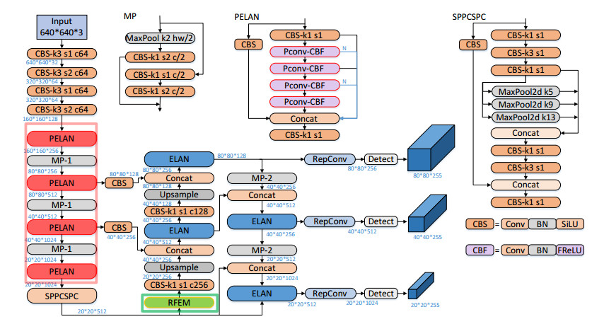
In daily life, snail classification is an important mean to ensure food safety and prevent the occurrence of situations that toxic snails are mistakenly consumed. However, the current methods for snail classification are mostly based on manual labor, which is inefficient. Therefore, a snail detection and classification method based on improved YOLOv7 was proposed in this paper. First, in order to reduce the FLOPs of the model, the backbone of the original model was improved. Specifically, the original 3×3 regular convolution was replaced with 3×3 partial convolution, and the Conv2D_BN_SiLU module in the partial convolution was replaced with the Conv2D_BN_FReLU module. FReLU could enhance the model's representational capacity without increasing the number of parameters. Then, based on the specific features of snail images, in order to solve the problems of small and dense targets of diverse shapes, a receptive field enhancement module was added to the head to learn the different receptive fields of the feature maps and enhance the feature pyramid representation. In addition, the CIoU was replaced with the WIoU to make the model pay more attention to targets at the edge or difficult-to-regress accurate bounding boxes. Finally, the images of nine common types of snails were collected, including the Pomacea canaliculata, the Viviparidae, the Nassariidae, and so on. These images were then labeled using LabelImg software to create a snail image dataset. Experiments were conducted based on the dataset, and the results showed that the proposed method demonstrated the best performance compared to other state-of-the-art methods.

| [1] |
W. Min, L. Liu, Y. Liu, M. Luo, S. Jiang, A survey on food image recognition, Chin. J. Comput., 45 (2022), 542–566. https://doi.org/10.11897/SP.J.1016.2022.00542 doi: 10.11897/SP.J.1016.2022.00542

|
| [2] | S. Sajadmanesh, S. Jafarzadeh, S. A. Ossia, H. R. Rabiee, H. Haddadi, Y. Mejova, et al., Kissing cuisines: Exploring worldwide culinary habits on the web, in Proceedings of the 26th international conference on world wide web companion. (2017), 1013–1021. https://doi.org/10.1145/3041021.3055137 |
| [3] |
J. Chung, J. Chung, W. Oh, Y. Yoo, W. G. Lee, H. Bang, A glasses-type wearable device for monitoring the patterns of food intake and facial activity, Sci. Rep., 7 (2017), 41690. https://doi.org/10.1038/srep41690 doi: 10.1038/srep41690
|
| [4] |
J. Yao, W. Jin, C. Gong, B. Jia, S. Sui, Y. Liang, et al., Distribution characteristics of tetrodotoxin in the coastal waters of China, Mar. Environ. Sci., 40 (2021), 161–166. https://doi.org/10.12111/j.mes.20190299 doi: 10.12111/j.mes.20190299
|
| [5] |
Q. Chen, C. Peng, F. Zhao, J. Li, B. Gao, Study on genetic diversity of cone snail in south china sea based on COI sequences, Genomics Appl. Biol., 39 (2020), 3955–3960. https://doi.org/10.13417/j.gab.039.003955 doi: 10.13417/j.gab.039.003955
|
| [6] | J. MacQueen. Some methods for classification and analysis of multivariate observations, in Proceedings of the fifth Berkeley symposium on mathematical statistics and probability, 1 (1967), 281–297. |
| [7] |
C. Cortes, V. Vapnik. Support-vector networks, Mach. Learn., 20 (1995), 273–297. https://doi.org/10.1023/A:1022627411411 doi: 10.1023/A:1022627411411
|
| [8] |
X. Mai, H. Zhang, X. Jia, M. Q. H. Meng, Faster R-CNN with classifier fusion for automatic detection of small fruits, IEEE Trans. Autom. Sci. Eng., 17 (2020), 1555–1569. https://doi.org/10.1109/TASE.2020.2964289 doi: 10.1109/TASE.2020.2964289
|
| [9] | J. Liu, M. Zhao, X.Guo, A fruit detection algorithm based on r-fcn in natural scene, in 2020 Chinese Control and Decision Conference (CCDC), (2020), 487–492. https://doi.org/10.1109/CCDC49329.2020.9163826 |
| [10] |
S. Villon, D. Mouillot, M. Chaumont, E. S. Darling, S. Villéger, A deep learning method for accurate and fast identification of coral reef fishes in underwater images, Ecolog. Inform., 48 (2018), 238–244. https://doi.org/10.7287/peerj.preprints.26818 doi: 10.7287/peerj.preprints.26818
|
| [11] |
Y. Feng, X. Tao, E. J. Lee, Classification of shellfish recognition based on improved faster r-cnn framework of deep learning, Math. Probl. Eng., 2021 (2021), 1–10. https://doi.org/10.1155/2021/1966848 doi: 10.1155/2021/1966848
|
| [12] | Z. Wang, I. Lee, Y. Tie, J. Cai, L. Qi, Real-world field snail detection and tracking, in 2018 15th International Conference on Control, Automation, Robotics and Vision (ICARCV), (2018), 1703–1708. https://doi.org/10.1109/ICARCV.2018.8581271 |
| [13] | J. R. I. Borreta, J. A. Bautista, A. N. Yumang, Snail Recognition Using YOLO, in 2022 IEEE International Conference on Artificial Intelligence in Engineering and Technology (ⅡCAIET), (2022), 1–6. https://doi.org/10.1109/ⅡCAIET55139.2022.9936736 |
| [14] | G. Agorku, S. Hernandez, M. Falquez, S. Poddar, K. Amankwah-Nkyi, Traffic cameras to detect inland waterway barge traffic: An application of machine learning, arXiv preprint arXiv: 2401.03070, (2024). |
| [15] |
Q. H. Cap, A. Fukuda, S. Kagiwada, H. Uga, N. Iwasaki, H. Iyatomi, Towards robust plant disease diagnosis with hard-sample re-mining strategy, Comput. Electron. Agric., 215 (2023), 108375. https://doi.org/10.1016/j.compag.2023.108375 doi: 10.1016/j.compag.2023.108375
|
| [16] | M. E. Haque, A. Rahman, I. Junaeid, S. U. Hoque, M. Paul, Rice leaf disease classification and detection using yolov5, (2022), arXiv preprint arXiv: 2209.01579. |
| [17] | A. Pundhir, D. Verma, P. Kumar, B. Raman, Region extraction-based approach for cigarette usage classification using deep learning, (2021), arXiv: 2103.12523. |
| [18] | R. Liu, Z. Ren, Application of Yolo on mask detection task, in 2021 IEEE 13th International Conference on Computer Research and Development (ICCRD), (2021), 130–136. https://doi.org/10.1109/ICCRD51685.2021.9386366 |
| [19] | C. Y. Wang, A. Bochkovskiy, H. Y. M. Liao, YOLOv7: Trainable bag-of-freebies sets new state-of-the-art for real-time object detectors, in Proceedings of the IEEE/CVF Conference on Computer Vision and Pattern Recognition, (2023), 7464–7475. https://doi.org/10.1109/CVPR52729.2023.00721 |
| [20] |
J. Chen, S. Kao, H. He, W. Zhuo, S. Wen, C. H. Lee, et al., Run, Don't walk: Chasing higher FLOPS for faster neural networks, in Proceedings of the IEEE/CVF Conference on Computer Vision and Pattern Recognition, (2023), 12021–12031. https://doi.org/10.1109/CVPR52729.2023.01157 doi: 10.1109/CVPR52729.2023.01157
|
| [21] | A. G. Howard, M. Zhu, B. Chen, D. Kalenichenko, W. Wang, T. Weyand, et al., Mobilenets: Efficient convolutional neural networks for mobile vision applications, (2017), arXiv preprint arXiv: 1704.04861. |
| [22] |
S. Elfwing, E. Uchibe, K. Doya, Sigmoid-weighted linear units for neural network function approximation in reinforcement learning, Neural Netw., 107 (2018), 3–11. https://doi.org/10.1016/j.neunet.2017.12.012 doi: 10.1016/j.neunet.2017.12.012
|
| [23] | N. Ma, X. Zhang, J. Sun, Funnel activation for visual recognition, in ECCV 2020: 16th European Conference on Computer Vision, (2020), 351–368. https://doi.org/10.1007/978-3-030-58621-8_21 |
| [24] | A. Krizhevsky, I. Sutskever, G. E. Hinton, Imagenet classification with deep convolutional neural networks, in 26th Annual Conference on Neural Information Processing Systems, NIPS 2012, Adv. Neural Inf. Proces. Syst., 25 (2012), 1097–1105. https://doi.org/10.1145/3065386 |
| [25] | X. Glorot, A. Bordes, Y. Bengio, Deep sparse rectifier neural networks, in Proceedings of the fourteenth international conference on artificial intelligence and statistics, J. Mach. Learn. Res., 15 (2011), 315–323. |
| [26] | Z. Yu, H. Huang, W. Chen, Y. Su, Y. Liu, X. Wang, Yolo-facev2: A scale and occlusion aware face detector, (2022), arXiv preprint arXiv: 2208.02019. |
| [27] | F. Yu, V. Koltun, Multi-scale context aggregation by dilated convolutions, (2015), arXiv preprint arXiv: 1511.07122. |
| [28] |
Z. Zheng, P. Wang, D. Ren, W. Liu, R. Ye, Q. Hu, et al., Enhancing geometric factors in model learning and inference for object detection and instance segmentation, IEEE Trans. Cybern., 52 (2021), 8574–8586. https://doi.org/10.1109/TCYB.2021.3095305 doi: 10.1109/TCYB.2021.3095305
|
| [29] | Z. Zheng, P. Wang, W. Liu, J. Li, R. Ye, D. Ren, Distance-IoU loss: Faster and better learning for bounding box regression, in Proceedings of the 34th AAAI conference on artificial intelligence, 34 (2020), 12993–13000. https://doi.org/10.1609/aaai.v34i07.6999 |
| [30] | Z. Tong, Y. Chen, Z. Xu, R. Yu, Wise-IoU: Bounding box regression loss with dynamic focusing mechanism, (2023), arXiv preprint arXiv: 2301.10051. |
| [31] | R. Padilla, S. L. Netto, E. A. B. Da Silva, A survey on performance metrics for object-detection algorithms, in Proceedings of the 2020 international conference on systems, signals and image processing (IWSSIP), (2020), 237–242. https://doi.org/10.1109/IWSSIP48289.2020.9145130 |
| [32] | C. Li, L. Li, H. Jiang, K. Weng, Y. Geng, L. Li, et al., YOLOv6: A single-stage object detection framework for industrial applications, (2022), arXiv preprint arXiv: 2209.02976. |
| [33] | Z. Ge, S. Liu, F. Wang, Z. Li, J. Sun, Yolox: Exceeding yolo series in 2021, (2021), arXiv preprint arXiv: 2107.08430. |
| [34] | W. Liu, D. Anguelov, D. Erhan, C. Szegedy, S. Reed, C. Fu, et al., SSD: Single shot multibox detector, in ECCV 2016: 14th European Conference on Computer Vision, (2016), 21–37. https://doi.org/10.1007/978-3-319-46448-0_2 |
| [35] |
S. Ren, K. He, R. Girshick, J. Sun, Faster r-cnn: Towards real-time object detection with region proposal networks, IEEE Trans. Pattern. Anal. Mach. Intell., 39 (2017), 1137–1149. https://doi.org/10.1109/TPAMI.2016.2577031 doi: 10.1109/TPAMI.2016.2577031
|
| [36] | T. Lin, P. Goyal, R. Girshick, K. He, P. Dollar, Focal loss for dense object detection, in Proceedings of the IEEE international conference on computer vision, (2017), 2980–2988. https://doi.org/10.1109/ICCV.2017.324 |


Figures(4) / Tables(5)

Qiming Li, Luoying Qiu. A snail species identification method based on deep learning in food safety[J]. Mathematical Biosciences and Engineering, 2024, 21(3): 3652-3667. doi: 10.3934/mbe.2024161


 DownLoad: