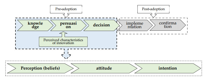
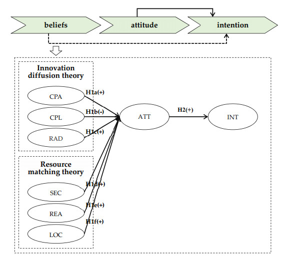
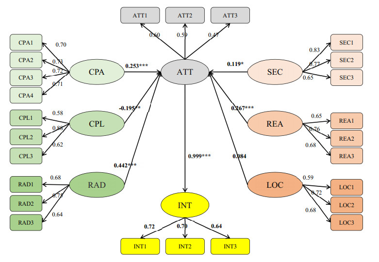
Self-service technology (SST) is a logistic innovation in e-commerce that enhances last-mile delivery efficiency in supply chain management. By combining Innovation Diffusion Theory with Resource Matching Theory, we proposed a comprehensive framework to explain the relationships between beliefs, attitude, and intention in Guanzhou, China. The findings revealed that attitude played a crucial role in influencing consumer intention to adopt SST and that attitude has direct and indirect effects. Additionally, consumer perceptions of compatibility, relative advantage, reliability, and complexity indirectly affected their adoption intention through attitude. These factors had positive and negative effects. The results highlighted the importance of attitudes as immediate predictors of intention, as consumer attitudes (favorable and unfavorable) were shaped by their perceptions. We conclude by recommending strategies to promote positive attitudes toward SST and enhance safety, efficiency, and the overall user experience.
Citation: Song Liu, Gusong Luo, Yonglong Cai, Wenjie Wu, Weitao Liu, Rong Zou, Wenxuan Tan. Determinants of consumer intention to adopt a self-service technology strategy for last-mile delivery in Guangzhou, China[J]. Mathematical Biosciences and Engineering, 2024, 21(2): 3262-3280. doi: 10.3934/mbe.2024144
Self-service technology (SST) is a logistic innovation in e-commerce that enhances last-mile delivery efficiency in supply chain management. By combining Innovation Diffusion Theory with Resource Matching Theory, we proposed a comprehensive framework to explain the relationships between beliefs, attitude, and intention in Guanzhou, China. The findings revealed that attitude played a crucial role in influencing consumer intention to adopt SST and that attitude has direct and indirect effects. Additionally, consumer perceptions of compatibility, relative advantage, reliability, and complexity indirectly affected their adoption intention through attitude. These factors had positive and negative effects. The results highlighted the importance of attitudes as immediate predictors of intention, as consumer attitudes (favorable and unfavorable) were shaped by their perceptions. We conclude by recommending strategies to promote positive attitudes toward SST and enhance safety, efficiency, and the overall user experience.

| [1] |
J. Visser, T. Nemoto, M. Browne M, Home delivery and the impacts on urban freight transport: A review, Proc. Soc. Behav. Sci., 125 (2014), 15–27. http://dx.doi.org/10.1016/j.sbspro.2014.01.1452 doi: 10.1016/j.sbspro.2014.01.1452

|
| [2] | EMarketer, UK Ecommerce Forecast 2023. Available from: https://www.insiderintelligence.com/content/uk-ecommerce-forecast-2023 |
| [3] |
E. Morganti, L. Dablanc, F. Fortin, Final deliveries for online shopping: The deployment of pickup point networks in urban and suburban areas, Res. Transp. Bus. Manage, 11 (2014), 23–31. http://dx.doi.org/10.1016/j.rtbm.2014.03.002 doi: 10.1016/j.rtbm.2014.03.002
|
| [4] | Ministry of Commerce, PRC: E-commerce in China 2022. Available from: http://dzsws.mofcom.gov.cn/article/ztxx/ndbg/202306/20230603415404.shtml |
| [5] |
L. B. Schewel, L. J. Schipper, Shop 'Till we drop: A historical and policy analysis of retail goods movement in the United States, Environ. Sci. Technol., 46 (2012), 9813–9821. http://dx.doi.org/10.1021/es301960f doi: 10.1021/es301960f
|
| [6] |
R. Gevaers, E. Van de Voorde, T. Vanelslander, Cost modelling and simulation of last-mile characteristics in an innovative B2C supply chain environment with implications on urban areas and cities, Proc. Soc. Behav. Sci., 125 (2014), 398–411. https://doi.org/10.1016/j.sbspro.2014.01.1483 doi: 10.1016/j.sbspro.2014.01.1483
|
| [7] |
J. R. Brown, A. L. Guiffrida, Carbon emissions comparison of last mile delivery versus customer pickup, Int. J. Logist. Resear., 17 (2014), 503–521. https://doi.org/10.1080/13675567.2014.907397 doi: 10.1080/13675567.2014.907397
|
| [8] |
D. Vyt, M. Jara, G. Cliquet, Grocery pickup creation of value: Customers' benefits vs. spatial dimension, J. Retailing Consum. Serv., 39 (2017), 145–153. https://doi.org/10.1016/j.jretconser.2017.08.004 doi: 10.1016/j.jretconser.2017.08.004
|
| [9] |
S. Iwan, K. Kijewska, J. Lemke, Analysis of parcel lockers' efficiency as the last mile delivery solution–the results of the research in Poland, Transp. Res. Procedia, 12 (2016), 644–655. https://doi.org/10.1016/j.trpro.2016.02.018 doi: 10.1016/j.trpro.2016.02.018
|
| [10] | State Post Bureau, Statistical Bulletin of the postal industry for 2022. Available from: https://www.spb.gov.cn/gjyzj/c100276/202305/d5756a12b51241a9b81dc841ff2122c6.shtml |
| [11] |
Y. Chen, J. Yu, S. Yang, J. Wei, Consumer's intention to use self-service parcel delivery service in online retailing, Int. Res., 28 (2018), 500–519. https://doi.org/10.1108/IntR-11-2016-0334 doi: 10.1108/IntR-11-2016-0334
|
| [12] | A. T. Collins, Behavioral influences on the environmental impact of collection/delivery points, in Green Logistics and Transportation (eds. B. Fahimnia, M. Bell, D. Hensher and J. Sarkis), Springer, (2015), 15–34. https://doi.org/10.1007/978-3-319-17181-4_2 |
| [13] |
J. C. Lin, H. Chang, The role of technology readiness in self-service technology acceptance, Manag. Serv. Qual. Int. J., 21 (2011), 424–444. https://doi.org/10.1108/09604521111146289 doi: 10.1108/09604521111146289
|
| [14] |
M. Blut, C. Wang, K. Schoefer, Factors influencing the acceptance of self-service technologies: A meta-analysis, J. Serv. Res., 19 (2016), 396–416. https://doi.org/10.1177/1094670516662 doi: 10.1177/1094670516662
|
| [15] |
K. F. Yuen, X. Wang, L. T. W. Ng, Y. D. Wong, An investigation of customers' intention to use self-collection services for last-mile delivery, Transp. Pol., 66 (2018), 1–8. https://doi.org/10.1016/j.tranpol.2018.03.001 doi: 10.1016/j.tranpol.2018.03.001
|
| [16] |
H. Oh, M. Jeong, S. Baloglu, Tourists' adoption of self-service technologies at resort hotels, J. Bus. Res., 66 (2013), 692–699. https://doi.org/10.1016/j.jbusres.2011.09.005 doi: 10.1016/j.jbusres.2011.09.005
|
| [17] |
X. Wang, K. F. Yuen, Y. D. Wong, C. C. Teo, An innovation diffusion perspective of e-consumers' initial adoption of self-collection service via automated parcel station, Int. J. Phys. Distr. Log., 29 (2018), 237–260. https://doi.org/10.1108/IJLM–12–2016–0302 doi: 10.1108/IJLM–12–2016–0302
|
| [18] |
K. F. Yuen, X. Wang, F. Ma, Y. D. Wong, The determinants of customers' intention to use smart lockers for last–mile deliveries, J. Retail. Consum. Serv., 49 (2019), 316–326. https://doi.org/10.1016/j.jretconser.2019.03.022 doi: 10.1016/j.jretconser.2019.03.022
|
| [19] |
J. Weltevreden, B2C e-commerce logistics: The rise of collection-and-delivery points in the Netherlands, Int. J. Retail Distrib. Manage., 36 (2008), 638–660. http://dx.doi.org/10.1108/09590550810883487 doi: 10.1108/09590550810883487
|
| [20] |
B. Motte-Baumvol, L. Belton-Chevallier, L. Dablanc, E. Morganti, C. Belin-Munier, Spatial dimensions of e-shopping in France, Asian Transp. Stud., 4 (2017), 585–600. http://dx.doi.org/10.11175/eastsats.4.585 doi: 10.11175/eastsats.4.585
|
| [21] |
I. O. Pappas, P. E. Kourouthanassis, M. N. Giannakos, V. Chrissikopoulos, Explaining online shopping behavior with fsQCA: The role of cognitive and affective perceptions, J. Bus. Res., 69 (2016), 794–803. https://doi.org/10.1016/j.jbusres.2015.07.010 doi: 10.1016/j.jbusres.2015.07.010
|
| [22] |
F. D. Davis, Perceived usefulness, perceived ease of use, and user acceptance of information technology, MIS Q., 13 (1989), 319–340. https://doi.org/10.2307/249008 doi: 10.2307/249008
|
| [23] |
X. Wang, K. F. Yuen, Y. D. Wong, C. C. Teo, Consumer participation in last-mile logistics service: An investigation on cognitions and affects, Int. J. Phys. Distr. Log., 49 (2019), 217–238. https://doi.org/10.1108/IJPDLM-12-2017-0372 doi: 10.1108/IJPDLM-12-2017-0372
|
| [24] |
Y. T. Tsai, P. Tiwasing, Customers' intention to adopt smart lockers in last-mile delivery service: A multi-theory perspective, J. Retail. Consum. Serv., 61 (2021), 102514. https://doi.org/10.1016/j.jretconser.2021.102514 doi: 10.1016/j.jretconser.2021.102514
|
| [25] |
M. Zhou, L. Zhao, N. Kong, K. S. Campy, G. Xu, G. Zhu, et al., Understanding consumers' behavior to adopt self–service parcel services for last–mile delivery, J. Retail. Consum. Serv., 52 (2020), 101911. https://doi.org/10.1016/j.jretconser.2019.101911 doi: 10.1016/j.jretconser.2019.101911
|
| [26] | C. Milioti, K. Pramatari, I. Kelepouri, Modelling consumers' acceptance for the click and collect service, J. Retail. Consum. Serv., 56 (2020) 102149. https://doi.org/10.1016/j.jretconser.2020.102149 |
| [27] |
A. Kedia, D. Kusumastuti, A. Nicholson, Acceptability of collection and delivery points from consumers' perspective: A qualitative case study of Christchurch city, Case Stud. Transp. Pol., 5 (2017), 587–595. https://doi.org/10.1016/j.cstp.2017.10.009 doi: 10.1016/j.cstp.2017.10.009
|
| [28] |
K. F. Yuen, V. V. Thai, Y. D. Wong, Are customers willing to pay for corporate social responsibility? A study of individual–specific mediators, Total Qual. Manag. Bus. Excel., 27 (2016), 912–926. https://doi.org/10.1080/14783363.2016.1187992 doi: 10.1080/14783363.2016.1187992
|
| [29] |
L. Festinger, A theory of cognitive dissonance, Am. J. Psychol., 72 (1957), 153–155. https://doi.org/10.2307/1420234 doi: 10.2307/1420234
|
| [30] |
R. J. Hill, M. Fishbein, I. Ajzen, Belief, attitude, intention and behavior: An introduction to theory and research, Contemp. Sociol., 6 (1977), 244. https://doi.org/10.2307/2065853 doi: 10.2307/2065853
|
| [31] | E. M. Rogers, Diffusion of Innovations, 4th edition, Free Press, New York, 1995. |
| [32] |
J. E. Collier, D. L. Sherrell, E. Babakus, A. B. Horky, Understanding the differences of public and private self-service technology, J. Serv. Mark., 28 (2014), 60–70. https://doi.org/10.1108/JSM-04-2012-0071 doi: 10.1108/JSM-04-2012-0071
|
| [33] |
J. M. Curran, M. L. Meuter, Self-service technology adoption: comparing three technologies, J. Serv. Mark., 19 (2005), 103–113. https://doi.org/10.1108/08876040510591411 doi: 10.1108/08876040510591411
|
| [34] |
G. Mortimer, L. Neale, S. F. E. Hasan, B. Dunphy, Investigating the factors influencing the adoption of m-banking: A cross-cultural study, Int. J. Bank Mark., 33 (2015), 545–570. https://doi.org/10.1108/IJBM-07-2014-0100 doi: 10.1108/IJBM-07-2014-0100
|
| [35] |
Z. Lin, R. Filieri, Airline passengers' continuance intention towards online check-in services: The role of personal innovativeness and subjective knowledge, Transp. Res. E Log., 81 (2015), 158–168. https://doi.org/10.1016/j.tre.2015.07.001 doi: 10.1016/j.tre.2015.07.001
|
| [36] |
R. Agarwal, J. Prasad, The role of innovation characteristics and perceived voluntariness in the acceptance of information technologies, Decis. Sci., 28 (1997), 557–582. https://doi.org/10.1111/j.1540-5915.1997.tb01322.x doi: 10.1111/j.1540-5915.1997.tb01322.x
|
| [37] |
V. Choudhury, E. Karahanna, The relative advantage of electronic channels: A multidimensional view, MIS Quart., 32 (2008), 179–200. https://doi.org/10.2307/25148833 doi: 10.2307/25148833
|
| [38] |
J. E. Collier, S. E. Kimes, Only if it is convenient: understanding how convenience influences self-service technology evaluation, J. Serv. Res. US, 16 (2012), 39–51. https://doi.org/10.1177/1094670512458454 doi: 10.1177/1094670512458454
|
| [39] | E. Karahanna, D. W. Straub, N. L. Chervany, Information technology adoption across time: A cross-sectional comparison of pre-adoption and post-adoption beliefs, MIS Quart., 23 (1999), 183–213. |
| [40] |
S. Taylor, P. Todd, Decomposition and crossover effects in the theory of planned behavior: A study of consumer adoption intention, Int. J. Res. Mark., 12 (1995), 137–155. https://doi.org/10.1016/0167-8116(94)00019-K doi: 10.1016/0167-8116(94)00019-K
|
| [41] |
A. Jeyaraj, J. Rottman, M. Lacity, A review of the predictors, linkages, and biases in IT innovation adoption research, J. Inf. Technol., 21 (2006), 1–23. https://doi.org/10.1057/palgrave.jit.2000056 doi: 10.1057/palgrave.jit.2000056
|
| [42] |
J. Khalilzadeh, A. B. Ozturk, A. Bilgihan, Security-related factors in extended UTAUT model for NFC based mobile payment in the restaurant industry, Comput. Hum. Behav., 70 (2017), 460–474. https://doi.org/10.1016/j.chb.2017.01.001 doi: 10.1016/j.chb.2017.01.001
|
| [43] |
D. Zhang, P. Zhu, Y. Ye, The effects of e-commerce on the demand for commercial real estate, Cities, 51 (2016), 106–120. https://doi.org/10.1016/j.cities.2015.11.012 doi: 10.1016/j.cities.2015.11.012
|
| [44] |
N. T. M. Demoulin, S. Djelassi, An integrated model of self-service technology (SST) usage in a retail context, Int. J. Retail. Distrib., 44 (2016), 540–559. https://doi.org/10.1108/IJRDM-08-2015-0122 doi: 10.1108/IJRDM-08-2015-0122
|
| [45] |
J. E. Collier, R. S. Moore, A. Horky, M. L. Moore, Why the little things matter: Exploring situational influences on customers' self-service technology decisions, J. Bus. Res., 68 (2015), 703–710. https://doi.org/10.1016/j.jbusres.2014.08.001 doi: 10.1016/j.jbusres.2014.08.001
|
| [46] |
P. Anand, B. Sternthal, Ease of message processing as a moderator of repetition effects in advertising, J. Mark. Res., 27 (1990), 345–353. https://doi.org/10.2307/3172591 doi: 10.2307/3172591
|
| [47] |
M. A. Jones, D. L. Mothersbaugh, S. E. Beatty, The effects of locational convenience on customer repurchase intentions across service types, J. Serv. Mark., 17 (2003), 701–712. https://doi.org/10.1108/08876040310501250 doi: 10.1108/08876040310501250
|
| [48] |
A. Parasuraman, Technology readiness index (TRI): A multiple-item scale to measure readiness to embrace new technologies, J. Serv. Res. US, 2 (2000), 307–320. https://doi.org/10.1177/109467050024001 doi: 10.1177/109467050024001
|
| [49] |
C. H. Lin, H. Y. Shih, P. Sher, Integrating technology readiness into technology acceptance: The TRAM model, Psychol. Market., 24 (2007), 641–657. https://doi.org/10.1002/mar.20177 doi: 10.1002/mar.20177
|
| [50] |
B. A. Martin, M. J. Sherrard, D. Wentzel, The role of sensation seeking and need for cognition on website evaluations: A resource-matching perspective, Psychol. Market., 22 (2005), 109–126. https://doi.org/10.1002/mar.20050 doi: 10.1002/mar.20050
|
| [51] | C. F. Chen, C. White, Y. E. Hsieh, The role of consumer participation readiness in automated parcel station usage intentions, J. Retail. Consum. Serv., 54 (2020). https://doi.org/10.1016/j.jretconser.2020.102063 |
Figures(3) / Tables(6)

Song Liu, Gusong Luo, Yonglong Cai, Wenjie Wu, Weitao Liu, Rong Zou, Wenxuan Tan. Determinants of consumer intention to adopt a self-service technology strategy for last-mile delivery in Guangzhou, China[J]. Mathematical Biosciences and Engineering, 2024, 21(2): 3262-3280. doi: 10.3934/mbe.2024144


 DownLoad: