Lung adenocarcinoma, a chronic non-small cell lung cancer, needs to be detected early. Tumor gene expression data analysis is effective for early detection, yet its challenges lie in a small sample size, high dimensionality, and multi-noise characteristics. In this study, we propose a lung adenocarcinoma convolutional neural network (LATCNN), a deep learning model tailored for accurate lung adenocarcinoma prediction and identification of key genes. During the feature selection stage, we introduce a hybrid algorithm. Initially, the fast correlation-based filter (FCBF) algorithm swiftly filters out irrelevant features, followed by applying the k-means-synthetic minority over-sampling technique (k-means-SMOTE) method to address category imbalance. Subsequently, we enhance the particle swarm optimization (PSO) algorithm by incorporating fast-decay dynamic inertia weights and utilizing the classification and regression tree (CART) as the fitness function for the second stage of feature selection, aiming to further eliminate redundant features. In the classifier construction stage, we present an attention convolutional neural network (atCNN) that incorporates an attention mechanism. This improved model conducts feature selection post lung adenocarcinoma gene expression data analysis for classification and prediction. The results show that LATCNN effectively reduces the feature dimensions and accurately identifies 12 key genes with accuracy, recall, F1 score, and MCC of 99.70%, 99.33%, 99.98%, and 98.67%, respectively. These performance metrics surpass those of other comparative models, highlighting the significance of this research for advancing lung adenocarcinoma treatment.
Citation: Kunpeng Li, Zepeng Wang, Yu Zhou, Sihai Li. Lung adenocarcinoma identification based on hybrid feature selections and attentional convolutional neural networks[J]. Mathematical Biosciences and Engineering, 2024, 21(2): 2991-3015. doi: 10.3934/mbe.2024133
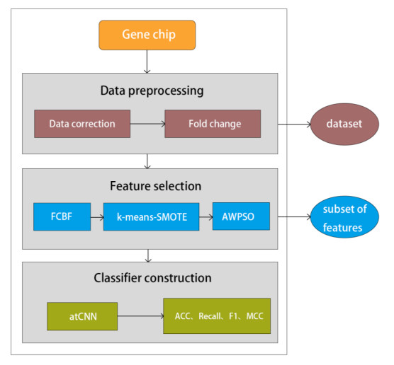
Lung adenocarcinoma, a chronic non-small cell lung cancer, needs to be detected early. Tumor gene expression data analysis is effective for early detection, yet its challenges lie in a small sample size, high dimensionality, and multi-noise characteristics. In this study, we propose a lung adenocarcinoma convolutional neural network (LATCNN), a deep learning model tailored for accurate lung adenocarcinoma prediction and identification of key genes. During the feature selection stage, we introduce a hybrid algorithm. Initially, the fast correlation-based filter (FCBF) algorithm swiftly filters out irrelevant features, followed by applying the k-means-synthetic minority over-sampling technique (k-means-SMOTE) method to address category imbalance. Subsequently, we enhance the particle swarm optimization (PSO) algorithm by incorporating fast-decay dynamic inertia weights and utilizing the classification and regression tree (CART) as the fitness function for the second stage of feature selection, aiming to further eliminate redundant features. In the classifier construction stage, we present an attention convolutional neural network (atCNN) that incorporates an attention mechanism. This improved model conducts feature selection post lung adenocarcinoma gene expression data analysis for classification and prediction. The results show that LATCNN effectively reduces the feature dimensions and accurately identifies 12 key genes with accuracy, recall, F1 score, and MCC of 99.70%, 99.33%, 99.98%, and 98.67%, respectively. These performance metrics surpass those of other comparative models, highlighting the significance of this research for advancing lung adenocarcinoma treatment.

| [1] | World Health Organization, Global health estimates 2020: Deaths by cause, age, sex, by country and by region, 2000–2019, Switzerland, (2020). |
| [2] | V. Gedvilaitė, E. Danila, S. Cicėnas, G. Smailytė, Lung cancer survival in Lithuania: changes by histology, age, and sex from 2003-2007 to 2008-2012, Cancer Control, 26 (2019). https://doi.org/10.1177/1073274819836085 |
| [3] |
K. Chansky, F. C. Detterbeck, A. G. Nicholson, V. W. Rusch, E. Vallières, P. Groome, et al., The IASLC lung cancer staging project: External validation of the revision of the TNM stage groupings in the eighth edition of the TNM classification of lung cancer, J. Thorac. Oncol., 12 (2017), 1109-1121. https://doi.org/10.1016/j.jtho.2017.04.011 doi: 10.1016/j.jtho.2017.04.011

|
| [4] |
T. Tamura, K. Kurishima, K. Nakazawa, K. Kagohashi, H. Ishikawa, H. Satoh, et al., Specific organ metastases and survival in metastatic non-small-cell lung cancer, Mol. Clin. Oncol., 3 (2014), 217-221. https://doi.org/10.3892/mco.2014.410 doi: 10.3892/mco.2014.410
|
| [5] |
G. Lightbody, V. Haberland, F. Browne, L. Taggart, H. Zheng, E. Parkes, et al., Review of applications of high-throughput sequencing in personalized medicine: Barriers and facilitators of future progress in research and clinical application, Brief. Bioinf., 20 (2019), 1795-1811. https://doi.org/10.1093/bib/bby051 doi: 10.1093/bib/bby051
|
| [6] |
F. S. Collins, H. Varmus, A new initiative on precision medicine, N. Engl. J. Med., 372 (2015), 793-795. https://doi.org/10.1056/NEJMp1500523 doi: 10.1056/NEJMp1500523
|
| [7] |
B. Vogelstein, N. Papadopoulos, V. E. Velculescu, S. B. Zhou, L. A. Diaz, K. W. Kinzler, Cancer genome landscapes, Science, 339 (2013), 1546-1558. https://doi.org/10.1126/science.1235122 doi: 10.1126/science.1235122
|
| [8] | L. Y. Chen, Z. J. Zhang, The self-distillation trained multitask dense-attention network for diagnosing lung cancers based on CT scans, Med. Phys., (2023). https://doi.org/10.1002/mp.16736 |
| [9] |
L. Y. Chen, H. Y. Qi, D. Lu, J. X. Zhai, K. K. Cai, L. Wang, et al., A deep learning based CT image analytics protocol to identify lung adenocarcinoma category and high-risk tumor area, STAR Protoc., 3 (2022), 101485. https://doi.org/10.1016/j.xpro.2022.101485 doi: 10.1016/j.xpro.2022.101485
|
| [10] |
L. Y. Chen, H. Y. Qi, D. Lu, J. X. Zhai, K. K. Cai, L. Wang, et al., Machine vision-assisted identification of the lung adenocarcinoma category and high-risk tumor area based on CT images, Patterns, 3 (2022), 100464. https://doi.org/10.1016/j.patter.2022.100464 doi: 10.1016/j.patter.2022.100464
|
| [11] |
L. Y. Gao, M. Q. Ye, C. R. Wu, Cancer classification based on support vector machine optimized by particle swarm optimization and artificial bee colony, Molecules, 22 (2017), 2086. https://doi.org/10.3390/molecules22122086 doi: 10.3390/molecules22122086
|
| [12] |
M. Yousef, A. Kumar, B. Bakir-Gungor, Application of biological domain knowledge based feature selection on gene expression data, Entropy, 23 (2020), 2. https://doi.org/10.3390/e23010002 doi: 10.3390/e23010002
|
| [13] |
J. Y. Xie, M. Z. Wang, Y. Zhou, H. C. Gao, S. Q. Xu, Differential expressed gene selection algorithms for unbalanced gene datasets, J. Comput., 42 (2019), 1232-1251. https://doi.org/10.11897/SP.J.1016.2019.01232 doi: 10.11897/SP.J.1016.2019.01232
|
| [14] |
M. Q. Ye, L. Y. Gao, C. R. Wu, C. Y Wan, Informative gene selection method based on symmetric uncertainty and SVM recursive feature elimination, Patt. Recog. Artif. Intell., 30 (2017), 429-438. https://doi.org/10.16451/j.cnki.issn1003-6059.201705005 doi: 10.16451/j.cnki.issn1003-6059.201705005
|
| [15] |
S. A. Ludwig, S. Picek, D. Jakobovic, Classification of cancer data: Analyzing gene expression data using a fuzzy decision tree algorithm, Oper. Res. Appl. Health Care Manage., 262 (2018), 327-347. https://doi.org/10.1007/978-3-319-65455-3_13 doi: 10.1007/978-3-319-65455-3_13
|
| [16] | D. Q. Zeebaree, H. Haron, A. M. Abdulazeez. Gene selection and classification of microarray data using convolutional neural network, in 2018 International Conference on Advanced Science and Engineering (ICOASE), (2018), 145-150. https://doi.org/10.1109/ICOASE.2018.8548836 |
| [17] |
T. Nguyen, A. Khosravi, D. Creighton, S. Nahavandi, A novel aggregate gene selection method for microarray data classification, Pat. Recog. Lett., 60 (2015), 16-23. https://doi.org/10.1016/j.patrec.2015.03.018 doi: 10.1016/j.patrec.2015.03.018
|
| [18] |
Y. W. Xiao, J. Wu, Z. L. Li, X. D. Zhao, A deep learning-based multi-model ensemble method for cancer prediction. Comput. Methods Programs Biomed., 153 (2018), 1-9. https://doi.org/10.1016/j.cmpb.2017.09.005 doi: 10.1016/j.cmpb.2017.09.005
|
| [19] |
G. Douzas, F. Bacao, F. Last, Improving imbalanced learning through a heuristic oversampling method based on k-means and SMOTE, Inf. Sci., 465 (2018), 1-20. https://doi.org/10.1016/j.ins.2018.06.056 doi: 10.1016/j.ins.2018.06.056
|
| [20] |
H. Okayama, T. Kohno, Y. Ishii, Y. Shimada, K. Shiraishi, R. Iwakawa, et al., Identification of genes upregulated in ALK-positive and EGFR/KRAS/ALK-negative lung adenocarcinomas, Cancer Res., 72 (2012), 100-111. https://doi.org/10.1158/0008-5472.CAN-11-1403 doi: 10.1158/0008-5472.CAN-11-1403
|
| [21] |
M. Yamauchi, R. Yamaguchi, A. Nakata, T. Kohno, M. Nagasaki, T. Shimamura, et al., Epidermal growth factor receptor tyrosine kinase defines critical prognostic genes of stage I lung adenocarcinoma, PLoS One, 7 (2012), e43923. https://doi.org/10.1371/journal.pone.0043923 doi: 10.1371/journal.pone.0043923
|
| [22] | X. H. Cao, I. Stojkovic, Z. Obradovic, A robust data scaling algorithm to improve classification accuracies in biomedical data, BMC Bioinf., 17 (2016). https://doi.org/10.1186/s12859-016-1236-x |
| [23] | L. Yu, H. Liu, Efficient feature selection via analysis of relevance and redundancy, J. Mach. Learn. Res., 5 (2004), 1205-1224. |
| [24] |
J. Liang, Z. Shi, D. Li, M. J. Wierman, Information entropy, rough entropy and knowledge granulation in incomplete information systems, Int. J. Gen. Syst., 35 (2006), 641-654. https://doi.org/10.1080/03081070600687668 doi: 10.1080/03081070600687668
|
| [25] |
L. M. Pan, M. H. Zhang, P. Ju, H. He, M. Ishii, Vertical co-current two-phase flow regime identification using fuzzy C-means clustering algorithm and ReliefF attribute weighting technique, Int. J. Heat Mass Transfer, 95 (2016), 393-404. https://doi.org/10.1016/j.ijheatmasstransfer.2015.11.081 doi: 10.1016/j.ijheatmasstransfer.2015.11.081
|
| [26] |
R. Sheikhpour, M. A. Sarram, R. Sheikhpour, Particle swarm optimization for bandwidth determination and feature selection of kernel density estimation based classifiers in diagnosis of breast cancer, Appl. Soft Comput., 40 (2016), 113-131. https://doi.org/10.1016/j.asoc.2015.10.005 doi: 10.1016/j.asoc.2015.10.005
|
| [27] |
M. Taherkhani, R. Safabakhsh, A novel stability-based adaptive inertia weight for particle swarm optimization, Appl. Soft Comput., 38 (2016), 281-295. https://doi.org/10.1016/j.asoc.2015.10.004 doi: 10.1016/j.asoc.2015.10.004
|
| [28] |
S. M. Vieira, L. F. Mendonca, G. J. Farinha, J. M. Sousa, Modified binary PSO for feature selection using SVM applied to mortality prediction of septic patients, Appl. Soft Comput., 13 (2013), 3494-3504. https://doi.org/10.1016/j.asoc.2013.03.021 doi: 10.1016/j.asoc.2013.03.021
|
| [29] | D. Ramyachitra, P. Manikandan, Imbalanced dataset classification and solutions: A review, Int. J. Comput. Bus. Res., 5 (2014). |
| [30] |
J. Wieczorek, C. Guerin, T. McMahon, K-fold cross-validation for complex sample surveys, Stat, 11 (2022), e454. https://doi.org/10.1002/sta4.454 doi: 10.1002/sta4.454
|
| [31] |
T. T. Li, H. P. Huang, G. Y. Shi, L. Y. Zhao, T. J. Li, Z. Zhang, et al., TGF-β1-SOX9 axis-inducible COL10A1 promotes invasion and metastasis in gastric cancer via epithelial-to-mesenchymal transition, Cell Death Dis., 9 (2018), 849. https://doi.org/10.1038/s41419-018-0877-2 doi: 10.1038/s41419-018-0877-2
|
| [32] |
Y. Zhong, L. T. Yang, F. Xiong, Y. He, Y. Y. Tang, L. Shi, et al., Long non-coding RNA AFAP1-AS1 accelerates lung cancer cells migration and invasion by interacting with SNIP1 to upregulate c-Myc, Signal Transduction Targeted Ther., 6 (2021), 240. https://doi.org/10.1038/s41392-021-00562-y doi: 10.1038/s41392-021-00562-y
|
| [33] |
Q. Q. Zhu, C. G. Zhang, T. Y. Qu, X. Y. Lu, X. Z. He, W. Li, et al., MNX1-AS1 promotes phase separation of IGF2BP1 to drive c-Myc–mediated cell-cycle progression and proliferation in lung cancer, Cancer Res., 82 (2022), 4340-4358. https://doi.org/10.1158/0008-5472.CAN-22-1289 doi: 10.1158/0008-5472.CAN-22-1289
|
| [34] |
Y. Z. Wu, J. M. Luo, H. Li, Y. Huang, Y. R. Zhu, Q. Q. Chen, B3GNT3 as a prognostic biomarker and correlation with immune cell infiltration in lung adenocarcinoma, Ann. Transl. Med., 10 (2022), 295. https://doi.org/10.21037/atm-22-493 doi: 10.21037/atm-22-493
|
| [35] |
Y. Y. Wang, M. Li, L. Zhang, Y. T. Chen, M. W. Ha, LINC01140 inhibits nonsmall cell lung cancer progression and cisplatin resistance through the miR-4742-5p/TACC1 axis, J. Biochem. Mol. Toxicol., 36 (2022), e23048. https://doi.org/10.1002/jbt.23048 doi: 10.1002/jbt.23048
|


Figures(10) / Tables(9)

Kunpeng Li, Zepeng Wang, Yu Zhou, Sihai Li. Lung adenocarcinoma identification based on hybrid feature selections and attentional convolutional neural networks[J]. Mathematical Biosciences and Engineering, 2024, 21(2): 2991-3015. doi: 10.3934/mbe.2024133


 DownLoad: