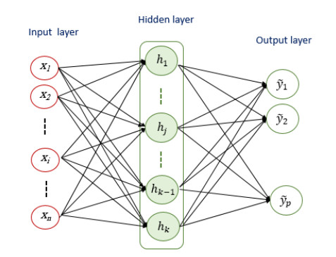
Training neural networks by using conventional supervised backpropagation algorithms is a challenging task. This is due to significant limitations, such as the risk for local minimum stagnation in the loss landscape of neural networks. That may prevent the network from finding the global minimum of its loss function and therefore slow its convergence speed. Another challenge is the vanishing and exploding gradients that may happen when the gradients of the loss function of the model become either infinitesimally small or unmanageably large during the training. That also hinders the convergence of the neural models. On the other hand, the traditional gradient-based algorithms necessitate the pre-selection of learning parameters such as the learning rates, activation function, batch size, stopping criteria, and others. Recent research has shown the potential of evolutionary optimization algorithms to address most of those challenges in optimizing the overall performance of neural networks. In this research, we introduce and validate an evolutionary optimization framework to train multilayer perceptrons, which are simple feedforward neural networks. The suggested framework uses the recently proposed evolutionary cooperative optimization algorithm, namely, the dynamic group-based cooperative optimizer. The ability of this optimizer to solve a wide range of real optimization problems motivated our research group to benchmark its performance in training multilayer perceptron models. We validated the proposed optimization framework on a set of five datasets for engineering applications, and we compared its performance against the conventional backpropagation algorithm and other commonly used evolutionary optimization algorithms. The simulations showed the competitive performance of the proposed framework for most examined datasets in terms of overall performance and convergence. For three benchmarking datasets, the proposed framework provided increases of 2.7%, 4.83%, and 5.13% over the performance of the second best-performing optimizers, respectively.
Citation: Rami AL-HAJJ, Mohamad M. Fouad, Mustafa Zeki. Evolutionary optimization framework to train multilayer perceptrons for engineering applications[J]. Mathematical Biosciences and Engineering, 2024, 21(2): 2970-2990. doi: 10.3934/mbe.2024132
Training neural networks by using conventional supervised backpropagation algorithms is a challenging task. This is due to significant limitations, such as the risk for local minimum stagnation in the loss landscape of neural networks. That may prevent the network from finding the global minimum of its loss function and therefore slow its convergence speed. Another challenge is the vanishing and exploding gradients that may happen when the gradients of the loss function of the model become either infinitesimally small or unmanageably large during the training. That also hinders the convergence of the neural models. On the other hand, the traditional gradient-based algorithms necessitate the pre-selection of learning parameters such as the learning rates, activation function, batch size, stopping criteria, and others. Recent research has shown the potential of evolutionary optimization algorithms to address most of those challenges in optimizing the overall performance of neural networks. In this research, we introduce and validate an evolutionary optimization framework to train multilayer perceptrons, which are simple feedforward neural networks. The suggested framework uses the recently proposed evolutionary cooperative optimization algorithm, namely, the dynamic group-based cooperative optimizer. The ability of this optimizer to solve a wide range of real optimization problems motivated our research group to benchmark its performance in training multilayer perceptron models. We validated the proposed optimization framework on a set of five datasets for engineering applications, and we compared its performance against the conventional backpropagation algorithm and other commonly used evolutionary optimization algorithms. The simulations showed the competitive performance of the proposed framework for most examined datasets in terms of overall performance and convergence. For three benchmarking datasets, the proposed framework provided increases of 2.7%, 4.83%, and 5.13% over the performance of the second best-performing optimizers, respectively.

| [1] | S. Haykin, Neural Networks and Learning Machines, Prentice Hall, 2011. |
| [2] | O. I. Abiodun, A. Jantan, A. E. Omolara, K. V. Dada, N. A. Mohamed, H. Arshad, State-of-the-art in artificial neural network applications: A survey, Heliyon, 4 (2018). https://doi.org/10.1016/j.heliyon.2018.e00938 |
| [3] |
F. Li, M. Sun, EMLP: Short-term gas load forecasting based on ensemble multilayer perceptron with adaptive weight correction, Math. Biosci. Eng., 18 (2021), 1590–1608. https://doi.org/10.3934/mbe.2021082 doi: 10.3934/mbe.2021082

|
| [4] | A. Rana, A. S. Rawat, A. Bijalwan, H. Bahuguna, Application of multi layer (perceptron) artificial neural network in the diagnosis system: a systematic review, in 2018 International Conference on Research in Intelligent and Computing in Engineering (RICE), (2018), 1–6. https://doi.org/10.1109/RICE.2018.8509069 |
| [5] |
L. C. Velasco, J. F. Bongat, C. Castillon, J. Laurente, E. Tabanao, Days-ahead water level forecasting using artificial neural networks for watersheds, Math. Biosci. Eng., 20 (2023), 758–774. https://doi.org/10.3934/mbe.2023035 doi: 10.3934/mbe.2023035
|
| [6] | S. Hochreiter, A. S. Younger, P. R. Conwell, Learning to learn using gradient descent, in Artificial Neural Networks—ICANN 2001: International Conference Vienna, (2001), 87–94. https://doi.org/10.1007/3-540-44668-0_13 |
| [7] |
L. M. Saini, M. K. Soni, Artificial neural network-based peak load forecasting using conjugate gradient methods, IEEE Trans. Power Syst., 17 (2002), 907–912. https://doi.org/10.1109/TPWRS.2002.800992 doi: 10.1109/TPWRS.2002.800992
|
| [8] |
H. Adeli, A. Samant, An adaptive conjugate gradient neural network-wavelet model for traffic incident detection, Comput. Aided Civil Infrast. Eng., 15 (2000), 251–260. https://doi.org/10.1111/0885-9507.00189 doi: 10.1111/0885-9507.00189
|
| [9] |
J. Bilski, B. Kowalczyk, A. Marchlewska, J. M. Zurada, Local Levenberg-Marquardt algorithm for learning feedforwad neural networks, J. Artif. Intell. Soft Comput. Res., 10 (2020), 299–316. https://doi.org/10.2478/jaiscr-2020-0020 doi: 10.2478/jaiscr-2020-0020
|
| [10] | R. Pascanu, T. Mikolov, T. Y. Bengio, On the difficulty of training recurrent neural networks, in International Conference on Machine Learning, (2013), 1310–1318. |
| [11] |
H. Faris, I. Aljarah, S. Mirjalili, Training feedforward neural networks using multi-verse optimizer for binary classification problems, Appl. Intell., 45 (2016), 322–332. https://doi.org/10.1007/s10489-016-0767-1 doi: 10.1007/s10489-016-0767-1
|
| [12] |
M. Črepinšek, S. H. Liu, M. Mernik, Exploration and exploitation in evolutionary algorithms: A survey, ACM Comput. Surv., 45 (2013), 1–33. https://doi.org/10.1145/2480741.2480752 doi: 10.1145/2480741.2480752
|
| [13] |
G. Xu, An adaptive parameter tuning of particle swarm optimization algorithm, Appl. Math. Comput., 219 (2013), 4560–4569. https://doi.org/10.1016/j.amc.2012.10.067 doi: 10.1016/j.amc.2012.10.067
|
| [14] |
S. Mirjalili, S. Z. M. Hashim, H. M. Sardroudi, Training feedforward neural networks using hybrid particle swarm optimization and gravitational search algorithm, Appl. Math. Comput., 218 (2012), 11125–11137. https://doi.org/10.1016/j.amc.2012.04.069 doi: 10.1016/j.amc.2012.04.069
|
| [15] | X. S. Yang, Random walks and optimization, in Nature Inspired Optimization Algorithms, Elsevier, (2014), 45–65. https://doi.org/10.1016/B978-0-12-416743-8.00003-8 |
| [16] |
M. Ghasemi, S. Ghavidel, S. Rahmani, A. Roosta, H. Falah, A novel hybrid algorithm of imperialist competitive algorithm and teaching learning algorithm for optimal power flow problem with non-smooth cost functions, Eng. Appl. Artif. Intell., 29 (2014), 54–69. https://doi.org/10.1016/j.engappai.2013.11.003 doi: 10.1016/j.engappai.2013.11.003
|
| [17] |
S. Pothiya, I. Ngamroo, W. Kongprawechnon, Ant colony optimisation for economic dispatch problem with non-smooth cost functions, Int. J. Electr. Power Energy Syst., 32 (2010), 478–487. https://doi.org/10.1016/j.ijepes.2009.09.016 doi: 10.1016/j.ijepes.2009.09.016
|
| [18] |
M. M. Fouad, A. I. El-Desouky, R. Al-Hajj, E. S. M. El-Kenawy, Dynamic group-based cooperative optimization algorithm, IEEE Access, 8 (2020), 148378–148403. https://doi.org/10.1109/ACCESS.2020.3015892 doi: 10.1109/ACCESS.2020.3015892
|
| [19] |
S. Mirjalili, S. M. Mirjalili, A. Lewis, Grey wolf optimizer, Adv. Eng. Software, 69 (2014), 46–61. https://doi.org/10.1016/j.advengsoft.2013.12.007 doi: 10.1016/j.advengsoft.2013.12.007
|
| [20] |
F. Van den Bergh, A. P. Engelbrecht, A cooperative approach to particle swarm optimization, IEEE Trans. Evol. Comput., 8 (2004), 225–239. https://doi.org/10.1109/TEVC.2004.826069 doi: 10.1109/TEVC.2004.826069
|
| [21] |
C. K. Goh, K. C. Tan, A competitive-cooperative co-evolutionary paradigm for dynamic multi-objective optimization, IEEE Trans. Evol. Comput., 13 (2008), 103–127. https://doi.org/10.1109/TEVC.2008.920671 doi: 10.1109/TEVC.2008.920671
|
| [22] | J. H. Holland, Adaptation in Natural and Artificial Systems, MIT Press, Cambridge, 1992. https://doi.org/10.7551/mitpress/1090.001.0001 |
| [23] | D. E. Goldberg, Genetic Algorithms in Search Optimization and Machine Learning, Addison-Wesley, 1989. |
| [24] | EK Burke, EK Burke, G Kendall, G Kendall, Search Methodologies: Introductory Tutorials in Optimization and Decision Support Techniques, Springer, 2014. https://doi.org/10.1007/978-1-4614-6940-7 |
| [25] | U. Seiffert, Multiple layer perceptron training using genetic algorithms, in Proceedings of the European Symposium on Artificial Neural Networks, (2001), 159–164. |
| [26] | F. Ecer, S. Ardabili, S. S. Band, A. Mosavi, Training multilayer perceptron with genetic algorithms and particle swarm optimization for modeling stock price index prediction, 22 (2020), Entropy, 1239. https://doi.org/10.3390/e22111239 |
| [27] |
C. Zanchettin, T. B. Ludermir, L. M. Almeida, Hybrid training method for MLP: Optimization of architecture and training, IEEE Trans. Syst. Man Cyber. Part B, 41 (2011), 1097–1109. https://doi.org/10.1109/TSMCB.2011.2107035 doi: 10.1109/TSMCB.2011.2107035
|
| [28] |
H. Wang, H. Moayedi, L. Kok Foong, Genetic algorithm hybridized with multilayer perceptron to have an economical slope stability design, Eng. Comput., 37 (2021), 3067–3078. https://doi.org/10.1007/s00366-020-00957-5 doi: 10.1007/s00366-020-00957-5
|
| [29] |
C. C. Ribeiro, P. Hansen, V. Maniezzo, A. Carbonaro, Ant colony optimization: An overview, Essay Sur. Metaheuristics, 2002 (2002), 469–492. https://doi.org/10.1007/978-1-4615-1507-4_21 doi: 10.1007/978-1-4615-1507-4_21
|
| [30] | M. Dorigo, T. Stützle, Ant Colony Optimization: Overview and Recent Advances, Springer International Publishing, (2019), 311–351. https://doi.org/10.1007/978-3-319-91086-4_10 |
| [31] |
D. Karaboga, B. Gorkemli, C. Ozturk, N. Karaboga, A comprehensive survey: Artificial bee colony (ABC) algorithm and applications, Artif. Intell. Revi., 42 (2014), 21–57. https://doi.org/10.1007/s10462-012-9328-0 doi: 10.1007/s10462-012-9328-0
|
| [32] |
B. A. Garro, R. A. Vázquez, Designing artificial neural networks using particle swarm optimization algorithms, Comput. Intell. Neurosci., 2015 (2015), 61. https://doi.org/10.1155/2015/369298 doi: 10.1155/2015/369298
|
| [33] | I. Vilovic, N. Burum, Z. Sipus, Ant colony approach in optimization of base station position, in 2009 3rd European Conference on Antennas and Propagation, (2009), 2882–2886. |
| [34] |
K. Socha, C. Blum, An ant colony optimization algorithm for continuous optimization: Application to feed-forward neural network training, Neural Comput. Appl., 16 (2007), 235–247. https://doi.org/10.1007/s00521-007-0084-z doi: 10.1007/s00521-007-0084-z
|
| [35] |
M. Mavrovouniotis, S. Yang, Training neural networks with ant colony optimization algorithms for pattern classification, Soft Comput., 19 (2015), 1511–1522. https://doi.org/10.1007/s00500-014-1334-5 doi: 10.1007/s00500-014-1334-5
|
| [36] | C. Ozturk, D. Karaboga, Hybrid artificial bee colony algorithm for neural network training, in 2011 IEEE Congress of Evolutionary Computation (CEC), (2011), 84–88. https://doi.org/10.1109/CEC.2011.5949602 |
| [37] |
R. Storn, K. Price, Differential evolution–a simple and efficient heuristic for global optimization over continuous spaces, J. Global Optimization, 11 (1997), 341–359. https://doi.org/10.1023/A:1008202821328 doi: 10.1023/A:1008202821328
|
| [38] |
N. Bacanin, K. Alhazmi, M. Zivkovic, K. Venkatachalam, T. Bezdan, J. Nebhen, Training multi-layer perceptron with enhanced brain storm optimization metaheuristics, Comput. Mater. Contin, 70 (2022), 4199–4215. https://doi.org/10.32604/cmc.2022.020449 doi: 10.32604/cmc.2022.020449
|
| [39] |
J. Ilonen, J. K. Kamarainen, J. Lampinen, Differential evolution training algorithm for feed-forward neural networks, Neural Process. Lett., 17 (2003), 93–105. https://doi.org/10.1023/A:1022995128597 doi: 10.1023/A:1022995128597
|
| [40] | A. Slowik, M. Bialko, Training of artificial neural networks using differential evolution algorithm, in 2008 Conference on Human System Interactions, (2008), 60–65. https://doi.org/10.1109/HSI.2008.4581409 |
| [41] |
A. A. Bataineh, D. Kaur, S. M. J. Jalali, Multi-layer perceptron training optimization using nature inspired computing, IEEE Access, 10 (2022), 36963–36977. https://doi.org/10.1109/ACCESS.2022.3164669 doi: 10.1109/ACCESS.2022.3164669
|
| [42] | K. N. Dehghan, S. R. Mohammadpour, S. H. A. Rahamti, US natural gas consumption analysis via a smart time series approach based on multilayer perceptron ANN tuned by metaheuristic algorithms, in Handbook of Smart Energy Systems, Springer International Publishing, (2023), 1–13. https://doi.org/10.1007/978-3-030-72322-4_137-1 |
| [43] |
A. Alimoradi, H. Hajkarimian, H. H. Ahooi, M. Salsabili, Comparison between the performance of four metaheuristic algorithms in training a multilayer perceptron machine for gold grade estimation, Int. J. Min. Geo-Eng., 56 (2022), 97–105. https://doi.org/10.22059/ijmge.2021.314154.594880 doi: 10.22059/ijmge.2021.314154.594880
|
| [44] |
K. Bandurski, W. Kwedlo, A Lamarckian hybrid of differential evolution and conjugate gradients for neural network training, Neural Process. Lett., 32 (2010), 31–44. https://doi.org/10.1007/s11063-010-9141-1 doi: 10.1007/s11063-010-9141-1
|
| [45] | B. Warsito, A. Prahutama, H. Yasin, S. Sumiyati, Hybrid particle swarm and conjugate gradient optimization in neural network for prediction of suspended particulate matter, in E3S Web of Conferences, (2019), 25007. https://doi.org/10.1051/e3sconf/201912525007 |
| [46] |
A. Cuk, T. Bezdan, N. Bacanin, M. Zivkovic, K. Venkatachalam, T. A. Rashid, et al., Feedforward multi-layer perceptron training by hybridized method between genetic algorithm and artificial bee colony, Data Sci. Data Anal. Oppor. Challenges, 2021 (2021), 279. https://doi.org/10.1201/9781003111290-17-21 doi: 10.1201/9781003111290-17-21
|
| [47] | UC Irvine Machine Learning Repository. Available form: http://archive.ics.uci.edu/ml/ |
| [48] | Kaggel Database. Available form: https://www.kaggle.com/datasets/ |
| [49] | F. Pedregosa, G. Varoquaux, A. Gramfort, V. Michel, B. Thirion, O. Grisel, et al., Scikit-learn: Machine learning in Python, J. Mach. Learn. Res., 12 (2011), 2825–2830. |
| [50] |
F. Dick, H. Tevaearai, Significance and limitations of the p value, Eur. J. Vasc. Endovascular Surg., 50 (2015), 815. https://doi.org/10.1016/j.ejvs.2015.07.026 doi: 10.1016/j.ejvs.2015.07.026
|


Figures(6) / Tables(6)

Rami AL-HAJJ, Mohamad M. Fouad, Mustafa Zeki. Evolutionary optimization framework to train multilayer perceptrons for engineering applications[J]. Mathematical Biosciences and Engineering, 2024, 21(2): 2970-2990. doi: 10.3934/mbe.2024132


 DownLoad: