With the growing number of user-side resources connected to the distribution system, an occasional imbalance between the distribution side and the user side arises, making short-term power load forecasting technology crucial for addressing this issue. To strengthen the capability of load multi-feature extraction and improve the accuracy of electric load forecasting, we have constructed a novel BILSTM-SimAM network model. First, the entirely non-recursive Variational Mode Decomposition (VMD) signal processing technique is applied to decompose the raw data into Intrinsic Mode Functions (IMF) with significant regularity. This effectively reduces noise in the load sequence and preserves high-frequency data features, making the data more suitable for subsequent feature extraction. Second, a convolutional neural network (CNN) mode incorporates Dropout function to prevent model overfitting, this improves recognition accuracy and accelerates convergence. Finally, the model combines a Bidirectional Long Short-Term Memory (BILSTM) network with a simple parameter-free attention mechanism (SimAM). This combination allows for the extraction of multi-feature from the load data while emphasizing the feature information of key historical time points, further enhancing the model's prediction accuracy. The results indicate that the R2 of the BILSTM-SimAM algorithm model reaches 97.8%, surpassing mainstream models such as Transformer, MLP, and Prophet by 2.0%, 2.7%, and 3.6%, respectively. Additionally, the remaining error metrics also show a reduction, confirming the validity and feasibility of the method proposed.
Citation: Mingju Chen, Fuhong Qiu, Xingzhong Xiong, Zhengwei Chang, Yang Wei, Jie Wu. BILSTM-SimAM: An improved algorithm for short-term electric load forecasting based on multi-feature[J]. Mathematical Biosciences and Engineering, 2024, 21(2): 2323-2343. doi: 10.3934/mbe.2024102
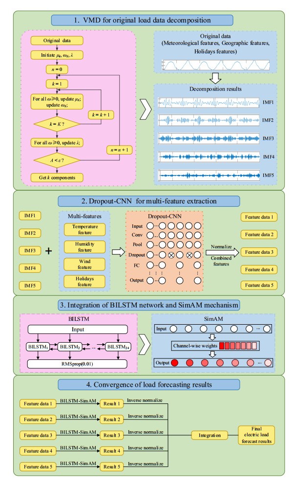
With the growing number of user-side resources connected to the distribution system, an occasional imbalance between the distribution side and the user side arises, making short-term power load forecasting technology crucial for addressing this issue. To strengthen the capability of load multi-feature extraction and improve the accuracy of electric load forecasting, we have constructed a novel BILSTM-SimAM network model. First, the entirely non-recursive Variational Mode Decomposition (VMD) signal processing technique is applied to decompose the raw data into Intrinsic Mode Functions (IMF) with significant regularity. This effectively reduces noise in the load sequence and preserves high-frequency data features, making the data more suitable for subsequent feature extraction. Second, a convolutional neural network (CNN) mode incorporates Dropout function to prevent model overfitting, this improves recognition accuracy and accelerates convergence. Finally, the model combines a Bidirectional Long Short-Term Memory (BILSTM) network with a simple parameter-free attention mechanism (SimAM). This combination allows for the extraction of multi-feature from the load data while emphasizing the feature information of key historical time points, further enhancing the model's prediction accuracy. The results indicate that the R2 of the BILSTM-SimAM algorithm model reaches 97.8%, surpassing mainstream models such as Transformer, MLP, and Prophet by 2.0%, 2.7%, and 3.6%, respectively. Additionally, the remaining error metrics also show a reduction, confirming the validity and feasibility of the method proposed.

| [1] |
I. S. Jahan, V. Snasel, S. Misak, Intelligent systems for power load forecasting: A study review, Energies, 13 (2020). https://doi.org/10.3390/en13226105 doi: 10.3390/en13226105

|
| [2] | A. K. Singh, S. Khatoon, M. Muazzam, D. Chaturvedi, Load forecasting techniques and methodologies: A review, in 2012 2nd International Conference on Power, Control and Embedded Systems, (2012), 1–10. https://doi.org/10.1109/ICPCES.2012.6508132 |
| [3] |
J. Zhu, H. Dong, W. Zheng, S. Li, Y. Huang, L. Xi, Review and prospect of data-driven techniques for load forecasting in integrated energy systems, Appl. Energy, 321 (2022). https://doi.org/10.1016/j.apenergy.2022.119269 doi: 10.1016/j.apenergy.2022.119269
|
| [4] |
N. Ahmad, Y. Ghadi, M. Adnan, M. Ali, Load forecasting techniques for power system: Research challenges and survey, IEEE Access, 10 (2022) 71054–71090. https://doi.org/10.1109/access.2022.3187839 doi: 10.1109/access.2022.3187839
|
| [5] |
R. Jiao, S. Wang, T. Zhang, H. Lu, H. He, B. B. Gupta, Adaptive feature selection and construction for day-ahead load forecasting use deep learning method, IEEE Trans. Netw. Serv. Manage., 18 (2021), 4019–4029. https://doi.org/10.1109/tnsm.2021.3110577 doi: 10.1109/tnsm.2021.3110577
|
| [6] |
H. L. Willis, J. E. Northcote-Green, Spatial electric load forecasting: A tutorial review, Proc. IEEE, 71 (1983), 232–253. https://doi.org/10.1109/tnsm.2021.3110577 doi: 10.1109/tnsm.2021.3110577
|
| [7] |
V. Azarova, D. Engel, C. Ferner, A. Kollmann, J. Reichl, Exploring the impact of network tariffs on household electricity expenditures using load profiles and socio-economic characteristics, Nat. Energy, 3 (2018), 317–325. https://doi.org/10.1038/s41560-018-0105-4 doi: 10.1038/s41560-018-0105-4
|
| [8] |
A. Ghasemi, H. Shayeghi, M. Moradzadeh, M. Nooshyar, A novel hybrid algorithm for electricity price and load forecasting in smart grids with demand-side management, Appl. Energy, 177 (2016), 40–59. https://doi.org/10.1016/j.apenergy.2016.05.083 doi: 10.1016/j.apenergy.2016.05.083
|
| [9] |
F. Ziel, Modeling public holidays in load forecasting: A German case study, J. Mod. Power Syst. Clean Energy, 6 (2018), 191–207. https://doi.org/10.1007/s40565-018-0385-5 doi: 10.1007/s40565-018-0385-5
|
| [10] |
F. M. Butt, L. Hussain, A. Mahmood, K. J. Lone, Artificial Intelligence based accurately load forecasting system to forecast short and medium-term load demands, Math. Biosci. Eng., 18 (2020), 400–425. https://doi.org/10.3934/mbe.2021022 doi: 10.3934/mbe.2021022
|
| [11] |
S. R. Khuntia, J. L. Rueda, M. A. van Der Meijden, Forecasting the load of electrical power systems in mid- and long-term horizons: A review, IET Gener. Transm. Distrib., 10 (2016), 3971–3977. https://doi.org/10.1049/iet-gtd.2016.0340 doi: 10.1049/iet-gtd.2016.0340
|
| [12] |
M. T. Hagan, S. M. Behr, The time series approach to short term load forecasting, IEEE Trans. Power Syst., 2 (1987), 785–791. https://doi.org/10.1109/TPWRS.1987.4335210 doi: 10.1109/TPWRS.1987.4335210
|
| [13] | T. Hong, and P. Wang, Fuzzy interaction regression for short term load forecasting. Fuzzy Optimization and Decision Making, 13 (2013) 91-103. https://doi.org/10.1007/s10700-013-9166-9 |
| [14] |
H. M. Al-Hamadi, S. A. Soliman, Fuzzy short-term electric load forecasting using Kalman filter, IEE Proc. Gener. Transm. Distrib., 153 (2006), 217–227. https://doi.org/10.1049/ip-gtd:20050088 doi: 10.1049/ip-gtd:20050088
|
| [15] |
J. W. Taylor, Short-term electricity demand forecasting using double seasonal exponential smoothing, J. Oper. Res. Soc., 54 (2017), 799–805. https://doi.org/10.1057/palgrave.jors.2601589 doi: 10.1057/palgrave.jors.2601589
|
| [16] |
J. W. Taylor, R. Buizza, Neural network load forecasting with weather ensemble predictions, IEEE Trans. Power Syst., 17 (2002), 626–632. https://doi.org/10.1109/TPWRS.2002.800906 doi: 10.1109/TPWRS.2002.800906
|
| [17] |
W. Sulandari, S. Subanar, M. H. Lee, P. C. Rodrigues, Indonesian electricity load forecasting using singular spectrum analysis, fuzzy systems and neural networks, Energy, 190 (2020). https://doi.org/10.1016/j.energy.2019.116408 doi: 10.1016/j.energy.2019.116408
|
| [18] |
V. Vlahović, I. Vujošević, Long-term forecasting: A critical review of direct-trend extrapolation methods, Int. J. Electr. Power Energy Syst., 9 (1987), 2–8. https://doi.org/10.1016/0142-0615(87)90019-6 doi: 10.1016/0142-0615(87)90019-6
|
| [19] | M. Lekshmi, K. A. Subramanya, Short-term load forecasting of 400 kV grid substation using R-tool and study of influence of ambient temperature on the forecasted load, in 2019 Second International Conference on Advanced Computational and Communication Paradigms (ICACCP), (2019), 1–5. https://doi.org/10.1109/ICACCP.2019.8883005 |
| [20] |
M. Mohandes, Support vector machines for short-term electrical load forecasting, Int. J. Energy Res., 26 (2002), 335–345. https://doi.org/10.1002/er.787 doi: 10.1002/er.787
|
| [21] |
Y. Dong, X. Ma, T. Fu, Electrical load forecasting: A deep learning approach based on K-nearest neighbors, Appl. Soft Comput., 99 (2021). https://doi.org/10.1016/j.asoc.2020.106900 doi: 10.1016/j.asoc.2020.106900
|
| [22] | Z. Xie, R. Wang, Z. Wu, T. Liu, Short-term power load forecasting model based on fuzzy neural network using improved decision tree, in 2019 IEEE Sustainable Power and Energy Conference (iSPEC), (2019), 482–486. https://doi.org/10.1109/iSPEC48194.2019.8975070 |
| [23] | G. Dudek, Short-term load forecasting using random forests, in Intelligent Systems'2014, Springer, (2015), 821–828. https://doi.org/10.1007/978-3-319-11310-47_1 |
| [24] |
K. B. Lindberg, P. Seljom, H. Madsen, D. Fischer, M. Korpås, Long-term electricity load forecasting: Current and future trends, Util. Policy, 58 (2019), 102–119. https://doi.org/10.1016/j.jup.2019.04.001 doi: 10.1016/j.jup.2019.04.001
|
| [25] | Z. A. Khan, A. Ullah, I. Ul Haq, M. Hamdy, G. M. Mauro, K. Muhammad, et al., Efficient short-term electricity load forecasting for effective energy management, Sustainable Energy Technol. Assess., 53 (2022). https://doi.org/10.1016/j.seta.2022.102337 |
| [26] | X. Sun, Z. Ouyang, D. Yue, Short-term load forecasting based on multivariate linear regression, in 2017 IEEE Conference on Energy Internet and Energy System Integration (EI2), (2017), 1–5. https://doi.org/10.1109/EI2.2017.8245401 |
| [27] |
X. Dong, S. Deng, D. Wang, A short-term power load forecasting method based on k-means and SVM, J. Ambient Intell. Hum. Comput., 13 (2021), 5253–5267. https://doi.org/10.1007/s12652-021-03444-x doi: 10.1007/s12652-021-03444-x
|
| [28] |
S. Fallah, M. Ganjkhani, S. Shamshirband, K. Chau, Computational intelligence on short-term load forecasting: A methodological overview, Energies, 12 (2019). https://doi.org/10.3390/en12030393 doi: 10.3390/en12030393
|
| [29] | A. Heydari, M. M. Nezhad, E. Pirshayan, D. A. Garcia, F. Keynia, L. De Santoli, Short-term electricity price and load forecasting in isolated power grids based on composite neural network and gravitational search optimization algorithm, Appl. Energy, 277 (2020). https://doi.org/10.1016/j.apenergy.2020.115503 |
| [30] |
M. Chen, Z. Lan, Z. Duan, S. Yi, Q. Su, HDS-YOLOv5: An improved safety harness hook detection algorithm based on YOLOv5s, Math. Biosci. Eng., 20 (2023), 15476–15495. https://doi.org/10.3934/mbe.2023691 doi: 10.3934/mbe.2023691
|
| [31] |
W. Zeng, J. Li, C. Sun, L. Cao, X. Tang, S. Shu, et al., Ultra short-term power load forecasting based on similar day clustering and ensemble empirical mode decomposition, Energies, 16 (2023). https://doi.org/10.3390/en16041989 doi: 10.3390/en16041989
|
| [32] |
X. Yan, M. Jia, Application of CSA-VMD and optimal scale morphological slice bispectrum in enhancing outer race fault detection of rolling element bearings, Mech. Syst. Signal Process., 122 (2019), 56–86.https://doi.org/10.1016/j.ymssp.2018.12.022 doi: 10.1016/j.ymssp.2018.12.022
|
| [33] | J. Chen, J. Zhang, A dual attention-based CNN-GRU model for short-term electric load forecasting, in The Proceedings of the 10th Frontier Academic Forum of Electrical Engineering (FAFEE2022), Springer, (2023), 715–725. https://doi.org/10.1007/978-981-99-3404-1_63 |
| [34] |
A. Wan, Q. Chang, K. Al-Bukhaiti, J. He, Short-term power load forecasting for combined heat and power using CNN-LSTM enhanced by attention mechanism, Energy, 282 (2023). https://doi.org/10.1016/j.energy.2023.128274 doi: 10.1016/j.energy.2023.128274
|
| [35] |
Q. Chen, W. Zhang, K. Zhu, D. Zhou, H. Dai, Q. Wu, A novel trilinear deep residual network with self-adaptive Dropout method for short-term load forecasting, Expert Syst. Appl., 182 (2021). https://doi.org/10.1016/j.eswa.2021.115272 doi: 10.1016/j.eswa.2021.115272
|
| [36] |
X. Ji, D. Liu, P. Xiong, Multi-model fusion short-term power load forecasting based on improved WOA optimization, Math. Biosci. Eng., 19 (2022), 13399–13420. https://doi.org/10.3934/mbe.2022627 doi: 10.3934/mbe.2022627
|
| [37] |
Z. Yao, T. Zhang, Q. Wang, Y. Zhao, R. Wang, Short-term power load forecasting of integrated energy system based on attention-CNN-DBILSTM, Math. Probl. Eng., 2022 (2022), 1–12. https://doi.org/10.1155/2022/1075698 doi: 10.1155/2022/1075698
|
| [38] |
K. Dragomiretskiy, D. Zosso, Variational Mode Decomposition, IEEE Trans. Signal Process., 62 (2014), 531–544. https://doi.org/10.1109/tsp.2013.2288675 doi: 10.1109/tsp.2013.2288675
|
| [39] | N. Srivastava, G. Hinton, A. Krizhevsky, I. Sutskever, R. Salakhutdinov, Dropout: A simple way to prevent neural networks from overfitting, J. Mach. Learn. Res., 15 (2014), 1929–1958. |
| [40] | Z. Huang, W. Xu, K. Yu, Bidirectional LSTM-CRF models for sequence tagging, arXiv preprint, (2015), arXiv: 1508.01991. https://doi.org/10.48550/arXiv.1508.01991 |
| [41] | L. Yang, R. Y. Zhang, L. Li, X. Xie, In SimAM: A simple, parameter-free attention module for convolutional neural networks, in International Conference on Machine Learning, PMLR, (2021), 11863–11874. https://icml.cc/virtual/2021/spotlight/8922 |


Figures(11) / Tables(6)

Mingju Chen, Fuhong Qiu, Xingzhong Xiong, Zhengwei Chang, Yang Wei, Jie Wu. BILSTM-SimAM: An improved algorithm for short-term electric load forecasting based on multi-feature[J]. Mathematical Biosciences and Engineering, 2024, 21(2): 2323-2343. doi: 10.3934/mbe.2024102


 DownLoad: