Simultaneous segmentation and classification of colon cancer polyp images using a dual branch multi-task learning network

Chenqian Li; Jun Liu; Jinshan Tang; Chenqian Li; Jun Liu; Jinshan Tang

doi:10.3934/mbe.2024090

Mathematical Biosciences and Engineering

2024, Volume 21, Issue 2: 2024-2049. doi: 10.3934/mbe.2024090

Previous Article Next Article

Research article Special Issues

Simultaneous segmentation and classification of colon cancer polyp images using a dual branch multi-task learning network

1.
School of Computer Science and Technology, Wuhan University of Science and Technology, Wuhan 430065, China
2.
Hubei Province Key Laboratory of Intelligent Information Processing and Real-Time Industrial System, Wuhan 430065, China
3.
Department of Health Administration and Policy, College of Public Health, George Mason University, Fairfax, VA 22030, USA

Academic Editor: Weining Wu

Received: 05 October 2023 Revised: 23 December 2023 Accepted: 26 December 2023 Published: 08 January 2024

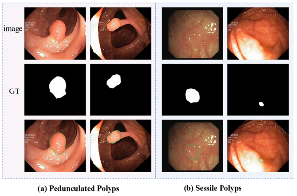
Accurate classification and segmentation of polyps are two important tasks in the diagnosis and treatment of colorectal cancers. Existing models perform segmentation and classification separately and do not fully make use of the correlation between the two tasks. Furthermore, polyps exhibit random regions and varying shapes and sizes, and they often share similar boundaries and backgrounds. However, existing models fail to consider these factors and thus are not robust because of their inherent limitations. To address these issues, we developed a multi-task network that performs both segmentation and classification simultaneously and can cope with the aforementioned factors effectively. Our proposed network possesses a dual-branch structure, comprising a transformer branch and a convolutional neural network (CNN) branch. This approach enhances local details within the global representation, improving both local feature awareness and global contextual understanding, thus contributing to the improved preservation of polyp-related information. Additionally, we have designed a feature interaction module (FIM) aimed at bridging the semantic gap between the two branches and facilitating the integration of diverse semantic information from both branches. This integration enables the full capture of global context information and local details related to polyps. To prevent the loss of edge detail information crucial for polyp identification, we have introduced a reverse attention boundary enhancement (RABE) module to gradually enhance edge structures and detailed information within polyp regions. Finally, we conducted extensive experiments on five publicly available datasets to evaluate the performance of our method in both polyp segmentation and classification tasks. The experimental results confirm that our proposed method outperforms other state-of-the-art methods.

Keywords:

Citation: Chenqian Li, Jun Liu, Jinshan Tang. Simultaneous segmentation and classification of colon cancer polyp images using a dual branch multi-task learning network[J]. Mathematical Biosciences and Engineering, 2024, 21(2): 2024-2049. doi: 10.3934/mbe.2024090

Related Papers:

[1]	Yinwan Cheng, Chao Yang, Bing Yao, Yaqin Luo . Neighbor full sum distinguishing total coloring of Halin graphs. AIMS Mathematics, 2022, 7(4): 6959-6970. doi: 10.3934/math.2022386
[2]	Baolin Ma, Chao Yang . Distinguishing colorings of graphs and their subgraphs. AIMS Mathematics, 2023, 8(11): 26561-26573. doi: 10.3934/math.20231357
[3]	Ningge Huang, Lily Chen . AVD edge-colorings of cubic Halin graphs. AIMS Mathematics, 2023, 8(11): 27820-27839. doi: 10.3934/math.20231423
[4]	Huifen Ge, Shumin Zhang, Chengfu Ye, Rongxia Hao . The generalized 4-connectivity of folded Petersen cube networks. AIMS Mathematics, 2022, 7(8): 14718-14737. doi: 10.3934/math.2022809
[5]	Kai An Sim, Kok Bin Wong . On the cooling number of the generalized Petersen graphs. AIMS Mathematics, 2024, 9(12): 36351-36370. doi: 10.3934/math.20241724
[6]	Fugang Chao, Donghan Zhang . Neighbor sum distinguishing total choice number of IC-planar graphs with restrictive conditions. AIMS Mathematics, 2023, 8(6): 13637-13646. doi: 10.3934/math.2023692
[7]	Bana Al Subaiei, Ahlam AlMulhim, Abolape Deborah Akwu . Vertex-edge perfect Roman domination number. AIMS Mathematics, 2023, 8(9): 21472-21483. doi: 10.3934/math.20231094
[8]	Yanyi Li, Lily Chen . Injective edge coloring of generalized Petersen graphs. AIMS Mathematics, 2021, 6(8): 7929-7943. doi: 10.3934/math.2021460
[9]	Ali Raza, Mobeen Munir, Tasawar Abbas, Sayed M Eldin, Ilyas Khan . Spectrum of prism graph and relation with network related quantities. AIMS Mathematics, 2023, 8(2): 2634-2647. doi: 10.3934/math.2023137
[10]	Bao-Hua Xing, Nurten Urlu Ozalan, Jia-Bao Liu . The degree sequence on tensor and cartesian products of graphs and their omega index. AIMS Mathematics, 2023, 8(7): 16618-16632. doi: 10.3934/math.2023850

Abstract

1. Preliminaries

Let $G$ be a simple, non-trivial connected graph with vertex set $V(G)$ . For any two distinct vertices $u$ and $v$ in $G$ , $u$ - $v$ geodesic is a shortest walk between $u$ and $v$ without repetition of vertices. Two vertices are said to be adjacent if there is an edge between them, and they are also called neighbors of each other. The collection of all the neighbors of a vertex $v$ in $G$ is called the (open) neighborhood of $v$ , denoted by $N(v)$ .

A vertex $v$ of $G$ distinguishes a pair $(x, y)$ of distinct vertices of $G$ , if the number of edges in $v$ - $x$ geodesic is different from the number of edge in $v$ - $y$ geodesic. If $(x, y)$ is a pair of neighbors in $G$ , then $v$ is said to be adjacently distinguish the pair $(x, y)$ . Equivalently, a vertex $v$ adjacently distinguishes a pair $(x, y)$ of two neighbors if the difference between the number of edges in $v$ - $x$ geodesic and the number of edges in $v$ - $y$ geodesic is one.

A set $D \subseteq V(G)$ is a distinguishing set (metric generator) for $G$ if the members of $D$ distinguish every pair of distinct vertices in $G$ . The cardinality of a smallest distinguishing set for $G$ is called the metric dimension of $G$ , denoted by $dim(G)$ ^[7,23]. The concept of distinguishing set was introduced, very firstly, by Blumenthal ^[5] in the general context of metric spaces. It was later rediscovered and studied, in the context of graphs, by Slater with the name locating set/reference set ^[23]. Independently, Harary and Melter studied distinguishing set as resolving set (metric generator) ^[7,20]. Applications of this notion to the navigation of robots in networks are discussed in ^[13,21], and applications to pharmaceutical chemistry in ^[10,11]. For more details about the theory and applications of this notion, we refer the readers to the papers cited in ^{[3,5,8,9,12,13,14,15,19,22]} and the references therein.

A set $A \subseteq V(G)$ is a neighbor-distinguishing set (local metric generator) for $G$ if the members of $A$ adjacently distinguish every pair of neighboring (adjacent) vertices in $G$ . The cardinality of a smallest neighbor-distinguishing set for $G$ is called the adjacency (local) metric dimension of $G$ , and we denote it by $dim_a(G)$ .

The problem of distinguishing every two neighbors with the aid of distance (the number of edges in a geodesic) in a connected graph was introduced and studied by Okamoto et al. in 2010 ^[16]. Then, up till now, this notion endlessly received remarkable interest of many researchers working with distance in graphs. In 2015 and 2018, every two neighbors in the corona product of graphs are distinguished ^[6,18], while this problem for strong product and lexicographic product of graphs was solved in 2016 ^[4] and in 2018 ^[2,6], respectively. Using the neighbor-distinguishing problem of primary subgraphs, this problem was solved for the super graphs of these subgraphs in 2015 ^[17]. In 2018, Salman et al. proposed linear programming formulation for this problem and distinguished neighbors in two families of convex polytopes ^[19]. Recently, in 2019, split graphs of complete and complete bipartite graphs have been considered in the context of this problem ^[1]. Due to this noteworthy attention of researchers to this problem, we extend this study towards a very renowned family of generalized Petersen graphs in this article. Next, we state two results, proved by Okamoto et al. ^[16], and Salman et al. ^[19], respectively, which will be used in the sequel.

Theorem 1. ^[16] Let $G$ be a non-trivial connected graph of order $n$ . Then $dim_a(G)$ $= n-1$ if and only if $G$ is a complete graph, and $dim_a(G) = 1$ if and only if $G$ is a bipartite graph.

Proposition 2. ^[19] A subset $A$ of vertices in a connected graph $G$ is a neighbor-distinguishing set for $G$ if and only if for every $u\in V(G)$ and for each $v\in N(u)$ , the pair $(u, v)$ adjacently distinguished by some element of $A$ .

Watkins, in $1969$ ^[24], generalized the eminent Petersen graph, and proposed the notation $P(n, m)$ to this generalized family, where $n \geq 3$ and $1 \leq m \leq \lfloor \frac{n-1}{2} \rfloor$ . $P(n, m)$ is a cubic graph having the set

$V(P(n, m)) = \{ u_{1} , u_{2} , \dots, u_{n} , v_{1} , v_{2} , \dots, v_{n} \}$

as the vertex set, and the set

$E(P(n, m)) = \bigcup\limits_{i = 1}^{n}\left\{u_ix, v_iy\; ;\; x\in N(u_i), \; y \in N(v_i)\right\}$

as the edge set, where $N(u_i) = \{u_{i+1}, u_{i-1}, v_i \}$ and $N(v_i) = \{u_i, v_{i+m}, v_{i-m} \}$ for each $1 \leq i \leq n$ , and the indices greater than $n$ or less than $1$ will be taken modulo $n$ . Vertices $u_i$ and $v_i$ $(1 \leq i \leq n)$ are called the outer vertices and inner vertices, respectively, in $P(n, m)$ . Figure 1 depicts graphs to two different families of generalized Petersen graphs.

Figure 1. Generalized Petersen graphs

$P(15, 4)$ and

$P(16, 7)$ .

DownLoad: Full-Size Img PowerPoint

The rest of the paper is divided into two sections: one is on the family of generalized Petersen graphs $P(n, 4)$ ; and the second is on the family of generalized Petersen graphs $P(2n, n-1)$ . These families have been considered in the context of metric dimension problem by Naz et al. ^[15] and Ahmad et al. ^[3], respectively. Here, we solve the neighbor-distinguishing problem for these families.

2. Family of generalized Petersen graphs $P(n, 4)$

In the next result, we show that only two vertices of $P(n, 4)$ perform the neighbor-distinguishing.

Theorem 3. For $n\geq 9$ , let $G$ be a generalized Petersen graph $P(n, 4)$ , then a neighbor-distinguishing set for $G$ is a $2$ -element subset of $V(G)$ .

Proof. For $n = 9$ , it is an easy exercise to see that the set $A = \{v_1, v_2 \}$ is a neighbor-distinguishing set for $G$ . For $n\geq 10$ , let $A$ be a $2$ -element subset of $V(G)$ . Then, according to Proposition 2, we would perform neighbor-distinguishing for each pair $(x, y)$ , where $x \in V(G)$ and $y \in N(x)$ . Note that, if $x \in A$ , then $(x, y)$ is adjacently distinguished, because the number of edges in $y-x$ geodesic is $1$ , while the number of edges in $x-x$ geodesic is $0$ . Now, we discuss the following eight cases:

Case 1: ( $n = 8k$ with $k\geq 2$ )

Let $A = \{v_1 = a_1, v_3 = a_2\}$ , then

● the number of edges in $u_1-a_2$ geodesic is 3,

● the number of edges in $u_2-a_2$ geodesic is 2,

● the number of edges in $v_1-a_2$ geodesic is 4,

● the number of edges in $v_2-a_2$ geodesic is 3.

Further, and provide the lists of number of edges in $x-a_1$ and $x-a_2$ geodesics for all $x \in V(G)-A$ .

Table 1. List of the number of edges in geodesics from the outer vertices to

$a \in A$ in

$P(n, 4)$ .

Geodesic	The number of edges in the geodesic
$u_i-a$	$i \equiv 0$ (mod 4)	$i \equiv 1$ (mod 4)	$i \equiv 2$ (mod 4)	$i \equiv 3$ (mod 4)
$n = 8k$ with $k\geq 2$ , and $A = \{v_1 = a_1, v_3 = a_2\}$
$u_i- a_1$ , $1\leq i \leq 4k+1$	$\frac{i+8}{4}$	$\frac{i+3}{4}$	$\frac{i+6}{4}$	$\frac{i+9}{4}$
$u_i- a_1$ , $4k+2\leq i \leq n$	$\frac{n-i+8}{4}$	$\frac{n-i+5}{4}$	$\frac{n-i+10}{4}$	$\frac{n-i+11}{4}$
$u_i- a_2$ , $3\leq i \leq 4k+3$	$\frac{i+4}{4}$	$\frac{i+7}{4}$	$\frac{i+6}{4}$	$\frac{i+1}{4}$
$u_i- a_2$ , $4k+4\leq i \leq n$	$\frac{n-i+12}{4}$	$\frac{n-i+13}{4}$	$\frac{n-i+10}{4}$	$\frac{n-i+7}{4}$
$n = 8k+1$ with $k\geq 2$ , and $A = \{v_1 = a_1, v_4 = a_2\}$
$u_i- a_1$ , $1\leq i \leq 4k+1$	$\frac{i+8}{4}$	$\frac{i+3}{4}$	$\frac{i+6}{4}$	$\frac{i+9}{4}$
$u_i- a_1$ , $4k+2\leq i \leq n$	$\frac{n-i+11}{4}$	$\frac{n-i+8}{4}$	$\frac{n-i+5}{4}$	$\frac{n-i+10}{4}$
$u_i- a_2$ , $4\leq i \leq 5k+1$	$\frac{i}{4}$	$\frac{i+3}{4}$	$\frac{i+6}{4}$	$\frac{i+5}{4}$
$u_i- a_2$ , $5k+2\leq i \leq n$	$\frac{n-i+11}{4}$	$\frac{n-i+8}{4}$	$\frac{n-i+13}{4}$	$\frac{n-i+14}{4}$
$n = 8k+2$ with $k\geq 1$ , and $A = \{v_1 = a_1, v_2 = a_2\}$
$u_i- a_1$ , $1\leq i \leq 4k+2$	$\frac{i+8}{4}$	$\frac{i+3}{4}$	$\frac{i+6}{4}$	$\frac{i+9}{4}$
$u_i- a_1$ , $4k+3\leq i \leq n$	$\frac{n-i+10}{4}$	$\frac{n-i+11}{4}$	$\frac{n-i+8}{4}$	$\frac{n-i+5}{4}$
$u_i- a_2$ , $2\leq i \leq 4k+3$	$\frac{i+8}{4}$	$\frac{i+7}{4}$	$\frac{i+2}{4}$	$\frac{i+5}{4}$
$u_i- a_2$ , $4k+4\leq i \leq n$	$\frac{n-i+6}{4}$	$\frac{n-i+11}{4}$	$\frac{n-i+12}{4}$	$\frac{n-i+9}{4}$
$n = 8k+3$ with $k\geq 1$ , and $A = \{v_1 = a_1, v_3 = a_2\}$
$u_i- a_1$ , $1\leq i \leq 4k+2$	$\frac{i+8}{4}$	$\frac{i+3}{4}$	$\frac{i+6}{4}$	$\frac{i+9}{4}$
$u_i- a_1$ , $4k+3\leq i \leq n$	$\frac{n-i+5}{4}$	$\frac{n-i+10}{4}$	$\frac{n-i+11}{4}$	$\frac{n-i+8}{4}$
$u_i- a_2$ , $3\leq i \leq 5k$	$\frac{i+4}{4}$	$\frac{i+7}{4}$	$\frac{i+6}{4}$	$\frac{i+1}{4}$
$u_i- a_2$ , $5k+1\leq i \leq n$	$\frac{n-i+13}{4}$	$\frac{n-i+10}{4}$	$\frac{n-i+7}{4}$	$\frac{n-i+12}{4}$
$n = 8k+4$ with $k\geq 1$ , and $A = \{v_1 = a_1, v_4 = a_2\}$
$u_i- a_1$ , $1\leq i \leq 4k+3$	$\frac{i+8}{4}$	$\frac{i+3}{4}$	$\frac{i+6}{4}$	$\frac{i+9}{4}$
$u_i- a_1$ , $4k+4\leq i \leq n$	$\frac{n-i+8}{4}$	$\frac{n-i+5}{4}$	$\frac{n-i+10}{4}$	$\frac{n-i+11}{4}$
$u_i- a_2$ , $3\leq i \leq 5k+2$	$\frac{i}{4}$	$\frac{i+3}{4}$	$\frac{i+6}{4}$	$\frac{i+5}{4}$
$u_i- a_2$ , $5k+3\leq i \leq n$	$\frac{n-i+8}{4}$	$\frac{n-i+13}{4}$	$\frac{n-i+14}{4}$	$\frac{n-i+11}{4}$
$n = 8k+5$ with $k\geq 1$ , and $A = \{v_1 = a_1, v_2 = a_2\}$
$u_i- a_1$ , $1\leq i \leq 5k+1$	$\frac{i+8}{4}$	$\frac{i+3}{4}$	$\frac{i+6}{4}$	$\frac{i+9}{4}$
$u_i- a_1$ , $5k+2\leq i \leq n$	$\frac{n-i+11}{4}$	$\frac{n-i+8}{4}$	$\frac{n-i+5}{4}$	$\frac{n-i+10}{4}$
$u_i- a_2$ , $2\leq i \leq 5k+2$	$\frac{i+8}{4}$	$\frac{i+7}{4}$	$\frac{i+2}{4}$	$\frac{i+5}{4}$
$u_i- a_2$ , $5k+3\leq i \leq n$	$\frac{n-i+11}{4}$	$\frac{n-i+12}{4}$	$\frac{n-i+9}{4}$	$\frac{n-i+6}{4}$
$n = 8k+6$ with $k\geq 1$ , and $A = \{v_1 = a_1, v_2 = a_2\}$
$u_i- a_1$ , $1\leq i \leq 4k+2$	$\frac{i+8}{4}$	$\frac{i+3}{4}$	$\frac{i+6}{4}$	$\frac{i+9}{4}$
$u_i- a_1$ , $4k+6\leq i \leq n$	$\frac{n-i+10}{4}$	$\frac{n-i+11}{4}$	$\frac{n-i+8}{4}$	$\frac{n-i+5}{4}$
$u_i- a_2$ , $1\leq i \leq 4k+3$	$\frac{i+8}{4}$	$\frac{i+7}{4}$	$\frac{i+2}{4}$	$\frac{i+5}{4}$
$u_i- a_2$ , $4k+7\leq i \leq n$	$\frac{n-i+6}{4}$	$\frac{n-i+11}{4}$	$\frac{n-i+12}{4}$	$\frac{n-i+9}{4}$
$n = 8k+7$ with $k\geq 1$ , and $A = \{v_1 = a_1, v_3 = a_2\}$
$u_i- a_1$ , $1\leq i \leq 4k+3$	$\frac{i+8}{4}$	$\frac{i+3}{4}$	$\frac{i+6}{4}$	$\frac{i+9}{4}$
$u_i- a_1$ , $4k+6\leq i \leq n$	$\frac{n-i+5}{4}$	$\frac{n-i+10}{4}$	$\frac{n-i+11}{4}$	$\frac{n-i+8}{4}$
$u_i- a_2$ , $2\leq i \leq 5k+1$	$\frac{i+4}{4}$	$\frac{i+7}{4}$	$\frac{i+6}{4}$	$\frac{i+1}{4}$
$u_i- a_2$ , $5k+4\leq i \leq n$	$\frac{n-i+13}{4}$	$\frac{n-i+10}{4}$	$\frac{n-i+7}{4}$	$\frac{n-i+12}{4}$

| Show Table

DownLoad: CSV

Table 2. List of the number of edges in geodesics from the inner vertices to

$a \in A$ in

$P(n, 4)$ .

Geodesic	The number of edges in the geodesic.
$v_i-a$	$i \equiv 0$ (mod 4)	$i \equiv 1$ (mod 4)	$i \equiv 2$ (mod 4)	$i \equiv 3$ (mod 4)
$n = 8k$ with $k\geq 2$ , and $A = \{v_1 = a_1, v_3 = a_2\}$
$v_i - a_1$ , $1\leq i \leq 4k+1$	$\frac{i+12}{4}$	$\frac{i-1}{4}$	$\frac{i+10}{4}$	$\frac{i+13}{4}$
$v_i - a_1$ , $4k+2\leq i \leq n$	$\frac{n-i+12}{4}$	$\frac{n-i+1}{4}$	$\frac{n-i+14}{4}$	$\frac{n-i+15}{4}$
$v_i - a_2$ , $3\leq i \leq 4k+3$	$\frac{i+8}{4}$	$\frac{i+11}{4}$	$\frac{i+10}{4}$	$\frac{i-3}{4}$
$v_i- a_2$ , $4k+4\leq i \leq n$	$\frac{n-i+16}{4}$	$\frac{n-i+17}{4}$	$\frac{n-i+14}{4}$	$\frac{n-i+3}{4}$
$n = 8k+1$ with $k\geq 2$ , and $A = \{v_1 = a_1, v_4 = a_2\}$
$v_i- a_1$ , $1\leq i \leq 3k+1$	$\frac{i+12}{4}$	$\frac{i-1}{4}$	$\frac{i+10}{4}$	$\frac{i+13}{4}$
$v_i- a_1$ , $3k+10\leq i \leq n$	$\frac{n-i+15}{4}$	$\frac{n-i+12}{4}$	$\frac{n-i+1}{4}$	$\frac{n-i+14}{4}$
$v_i- a_2$ , $4\leq i \leq 4k$	$\frac{i-4}{4}$	$\frac{i+7}{4}$	$\frac{i+10}{4}$	$\frac{i+9}{4}$
$v_i- a_2$ , $4k+6\leq i \leq n$	$\frac{n-i+15}{4}$	$\frac{n-i+4}{4}$	$\frac{n-i+17}{4}$	$\frac{n-i+18}{4}$
$n = 8k+2$ with $k\geq 1$ , and $A = \{v_1 = a_1, v_2 = a_2\}$
$v_i- a_1$ , $1\leq i \leq 3k+2$	$\frac{i+12}{4}$	$\frac{i-1}{4}$	$\frac{i+10}{4}$	$\frac{i+13}{4}$
$v_i- a_1$ , $3k+10\leq i \leq n$	$\frac{n-i+14}{4}$	$\frac{n-i+15}{4}$	$\frac{n-i+12}{4}$	$\frac{n-i+1}{4}$
$v_i- a_2$ , $2\leq i \leq 3k+3$	$\frac{i+12}{4}$	$\frac{i+11}{4}$	$\frac{i-2}{4}$	$\frac{i+9}{4}$
$v_i- a_2$ , $3k+11\leq i \leq n$	$\frac{n-i+2}{4}$	$\frac{n-i+15}{4}$	$\frac{n-i+16}{4}$	$\frac{n-i+13}{4}$
$n = 8k+3$ with $k\geq 1$ , and $A = \{v_1 = a_1, v_3 = a_2\}$
$v_i- a_1$ , $1\leq i \leq 3k+3$	$\frac{i+12}{4}$	$\frac{i-1}{4}$	$\frac{i+10}{4}$	$\frac{i+13}{4}$
$v_i- a_1$ , $3k+10\leq i \leq n$	$\frac{n-i+1}{4}$	$\frac{n-i+14}{4}$	$\frac{n-i+15}{4}$	$\frac{n-i+12}{4}$
$v_i- a_2$ , $3\leq i \leq 4k+1$	$\frac{i+8}{4}$	$\frac{i+11}{4}$	$\frac{i+10}{4}$	$\frac{i-3}{4}$
$v_i- a_2$ , $4k+8\leq i \leq n$	$\frac{n-i+17}{4}$	$\frac{n-i+14}{4}$	$\frac{n-i+3}{4}$	$\frac{n-i+16}{4}$
$n = 8k+4$ with $k\geq 1$ , and $A = \{v_1 = a_1, v_4 = a_2\}$
$v_i- a_1$ , $1\leq i \leq 4k+3$	$\frac{i+12}{4}$	$\frac{i-1}{4}$	$\frac{i+10}{4}$	$\frac{i+13}{4}$
$v_i- a_1$ , $4k+4\leq i \leq n$	$\frac{n-i+12}{4}$	$\frac{n-i+1}{4}$	$\frac{n-i+14}{4}$	$\frac{n-i+15}{4}$
$v_i- a_2$ , $3\leq i \leq 5k+2$	$\frac{i-4}{4}$	$\frac{i+7}{4}$	$\frac{i+10}{4}$	$\frac{i+9}{4}$
$v_i- a_2$ , $5k+3\leq i \leq n$	$\frac{n-i+4}{4}$	$\frac{n-i+17}{4}$	$\frac{n-i+18}{4}$	$\frac{n-i+15}{4}$
$n = 8k+5$ with $k\geq 1$ , and $A = \{v_1 = a_1, v_2 = a_2\}$
$v_i- a_1$ , $1\leq i \leq 4k+1$	$\frac{i+12}{4}$	$\frac{i-1}{4}$	$\frac{i+10}{4}$	$\frac{i+13}{4}$
$v_i- a_1$ , $4k+6\leq i \leq n$	$\frac{n-i+15}{4}$	$\frac{n-i+12}{4}$	$\frac{n-i+1}{4}$	$\frac{n-i+14}{4}$
$v_i- a_2$ , $2\leq i \leq 4k+2$	$\frac{i+12}{4}$	$\frac{i+11}{4}$	$\frac{i-2}{4}$	$\frac{i+9}{4}$
$v_i- a_2$ , $4k+7\leq i \leq n$	$\frac{n-i+15}{4}$	$\frac{n-i+16}{4}$	$\frac{n-i+13}{4}$	$\frac{n-i+2}{4}$
$n = 8k+6$ with $k\geq 1$ , and $A = \{v_1 = a_1, v_2 = a_2\}$
$v_i- a_1$ , $1\leq i \leq 3k+2$	$\frac{i+12}{4}$	$\frac{i-1}{4}$	$\frac{i+10}{4}$	$\frac{i+13}{4}$
$v_i- a_1$ , $3k+14\leq i \leq n$	$\frac{n-i+14}{4}$	$\frac{n-i+15}{4}$	$\frac{n-i+12}{4}$	$\frac{n-i+1}{4}$
$v_i- a_2$ , $1\leq i \leq 3k+3$	$\frac{i+12}{4}$	$\frac{i+11}{4}$	$\frac{i-2}{4}$	$\frac{i+9}{4}$
$v_i- a_2$ , $3k+15\leq i \leq n$	$\frac{n-i+2}{4}$	$\frac{n-i+15}{4}$	$\frac{n-i+16}{4}$	$\frac{n-i+13}{4}$
$n = 8k+7$ with $k\geq 1$ , and $A = \{v_1 = a_1, v_3 = a_2\}$
$v_i- a_1$ , $1\leq i \leq 3k+3$	$\frac{i+12}{4}$	$\frac{i-1}{4}$	$\frac{i+10}{4}$	$\frac{i+13}{4}$
$v_i- a_1$ , $3k+14\leq i \leq n$	$\frac{n-i+1}{4}$	$\frac{n-i+14}{4}$	$\frac{n-i+15}{4}$	$\frac{n-i+12}{4}$
$v_i- a_2$ , $2\leq i \leq 4k+1$	$\frac{i+8}{4}$	$\frac{i+11}{4}$	$\frac{i+10}{4}$	$\frac{i-3}{4}$
$v_i- a_2$ , $4k+12\leq i \leq n$	$\frac{n-i+17}{4}$	$\frac{n-i+14}{4}$	$\frac{n-i+3}{4}$	$\frac{n-i+16}{4}$

| Show Table

DownLoad: CSV

Case 2: ( $n = 8k+1$ with $k\geq 2$ )

Let $A = \{v_1 = a_1, v_4 = a_2\}$ , then

● the number of edges in $u_1-a_2$ geodesic is 3,

● the number of edges in $u_2-a_2$ geodesic is 3,

● the number of edges in $u_3-a_2$ geodesic is 2.

Further, – provide the lists of number of edges in $x-a_1$ and $x-a_2$ geodesics for all $x \in V(G)-A$ .

Table 3.

$\lambda_i$ is the number of edges in a

$v_i-a_1$ geodesic, and

$\lambda_j$ is the number of edges in a

$v_j-a_2$ geodesic.

$i$	$3k+2 \equiv 2 (mod \ 4)$	$3k+3 \equiv 3 (mod \ 4)$	$3k+4 \equiv 0 (mod \ 4)$	$3k+5 \equiv 1 (mod \ 4)$	$3k+6 \equiv 2 (mod \ 4)$	$3k+7 \equiv 3 (mod \ 4)$	$3k+8 \equiv 0 (mod \ 4)$	$3k+9 \equiv 1 (mod \ 4)$
$\lambda_i$	$\frac{5k}{4}$	$\frac{3k+16}{4}$	$\frac{3k+16}{4}$	$\frac{3k+4}{4}$	$\frac{5k-4}{4}$	$\frac{5k+8}{4}$	$\frac{5k+8}{4}$	$\frac{3k+8}{4}$
$j$	$1$	$2$	$3$	$4k+1 \equiv 1 (mod \ 4)$	$4k+2 \equiv 2 (mod \ 4)$	$4k+3 \equiv 3 (mod \ 4)$	$4k+4 \equiv 0 (mod \ 4)$	$4k+5 \equiv 1 (mod \ 4)$
$\lambda_j$	$4$	$4$	$3$	$k+1$	$k+3$	$k+3$	$k$	$k$

| Show Table

DownLoad: CSV

Case 3: ( $n = 8k+2$ with $k\geq 1$ )

Let $A = \{v_1 = a_1, v_2 = a_2\}$ , then

● the number of edges in $u_2-a_2$ geodesic is 2.

Further, , and provide the lists of number of edges in $x-a_1$ and $x-a_2$ geodesics for all $x \in V(G)-A$ .

Table 4.

$\lambda_i$ is the number of edges in a

$v_i-a_1$ geodesic, and

$\lambda_j$ is the number of edges in a

$v_j-a_2$ geodesic.

$i$	$3k+3 \equiv 3 (mod \ 4)$	$3k+4 \equiv 0 (mod \ 4)$	$3k+5 \equiv 1 (mod \ 4)$	$3k+6 \equiv 2 (mod \ 4)$	$3k+7 \equiv 3 (mod \ 4)$	$3k+8 \equiv 0 (mod \ 4)$	$3k+9 \equiv 1 (mod \ 4)$	$-$	$-$
$\lambda_i$	$\frac{5k}{4}$	$\frac{3k+16}{4}$	$\frac{3k+4}{4}$	$\frac{3k+16}{4}$	$\frac{5k-4}{4}$	$\frac{5k+8}{4}$	$\frac{3k+8}{4}$	$-$	$-$
$j$	$1$	$2$	$3k+4 \equiv 0 (mod \ 4)$	$3k+5 \equiv 1 (mod \ 4)$	$3k+6 \equiv 2 (mod \ 4)$	$3k+7 \equiv 3 (mod \ 4)$	$3k+8 \equiv 0 (mod \ 4)$	$3k+9 \equiv 1 (mod \ 4)$	$3k+10 \equiv 2 (mod \ 4)$
$\lambda_j$	$3$	$0$	$\frac{5k}{4}$	$\frac{3k+16}{4}$	$\frac{3k+4}{4}$	$\frac{5k+8}{4}$	$\frac{5k-4}{4}$	$\frac{5k+8}{4}$	$\frac{3k+8}{4}$

| Show Table

DownLoad: CSV

Case 4: ( $n = 8k+3$ with $k\geq 1$ )

Let $A = \{v_1 = a_1, v_3 = a_2\}$ , then

● the number of edges in $u_1-a_2$ geodesic is 3,

● the number of edges in $u_2-a_2$ geodesic is 2.

Further, , and provide the lists of number of edges in $x-a_1$ and $x-a_2$ geodesics for all $x \in V(G)-A$ .

Table 5.

$\lambda_i$ is the number of edges in a

$v_i-a_1$ geodesic, and

$\lambda_j$ is the number of edges in a

$v_j-a_2$ geodesic.

$i$	$3k+4 \equiv 0 (mod \ 4)$	$3k+5 \equiv 1 (mod \ 4)$	$3k+6 \equiv 2 (mod \ 4)$	$3k+7 \equiv 3 (mod \ 4)$	$3k+8 \equiv 0 (mod \ 4)$	$3k+9 \equiv 1 (mod \ 4)$	$-$	$-$
$\lambda_i$	$\frac{5k}{4}$	$\frac{3k+4}{4}$	$\frac{3k+16}{4}$	$\frac{5k+8}{4}$	$\frac{5k-4}{4}$	$\frac{3k+8}{4}$	$-$	$-$
$j$	$1$	$2$	$4k+2 \equiv 2 (mod \ 4)$	$4k+3 \equiv 3 (mod \ 4)$	$4k+4 \equiv 0 (mod \ 4)$	$4k+5 \equiv 1 (mod \ 4)$	$4k+6 \equiv 2 (mod \ 4)$	$4k+7\equiv 3 (mod \ 4)$
$\lambda_j$	$4$	$3$	$k+1$	$k$	$k+3$	$k+3$	$k$	$k+1$

| Show Table

DownLoad: CSV

Case 5: ( $n = 8k+4$ with $k\geq 1$ )

Let $A = \{v_1 = a_1, v_4 = a_2\}$ , then

● the number of edges in $v_1-a_2$ geodesic is 4,

● the number of edges in $v_2-a_2$ geodesic is 4,

● the number of edges in $u_1-a_2$ geodesic is 3,

● the number of edges in $u_2-a_2$ geodesic is 3.

Moreover, and provide the lists of number of edges in $x-a_1$ and $x-a_2$ geodesics for all $x \in V(G)-A$ .

Case 6: ( $n = 8k+5$ with $k\geq 1$ )

Let $A = \{v_1 = a_1, v_2 = a_2\}$ , then

● the number of edges in $u_1-a_2$ geodesic is 2,

● the number of edges in $v_1-a_2$ geodesic is 3.

Further, , and provide the lists of number of edges in $x-a_1$ and $x-a_2$ geodesics for all $x \in V(G)-A$ .

Table 6.

$\lambda_i$ is the number of edges in a

$v_i-a_1$ geodesic, and

$\lambda_j$ is the number of edges in a

$v_j-a_2$ geodesic.

$i$	$4k+2 \equiv 2 (mod \ 4)$	$4k+3 \equiv 3 (mod \ 4)$	$4k+4 \equiv 0 (mod \ 4)$	$4k+5 \equiv 1 (mod \ 4)$
$\lambda_i$	$k+1$	$k+4$	$k+4$	$k+1$
$j$	$4k+3 \equiv 3 (mod \ 4)$	$4k+4 \equiv 0 (mod \ 4)$	$4k+5 \equiv 1 (mod \ 4)$	$4k+6 \equiv 2 (mod \ 4)$
$\lambda_j$	$k+1$	$k+4$	$k+4$	$k+1$

| Show Table

DownLoad: CSV

Case 7: ( $n = 8k+6$ with $k\geq 1$ )

Let $A = \{v_1 = a_1, v_2 = a_2\}$ , then

● the number of edges in $v_{3k+3}-a_1$ geodesic is $\frac{5k+4}{4} \equiv 3 (mod \ 4)$ ,

● the number of edges in $v_{3k+4}-a_2$ geodesic is $\frac{5k+4}{4} \equiv 0 (mod \ 4)$ ,

● the number of edges in $u_{4k+3}-a_1$ geodesic is $k+2$ ,

● the number of edges in $u_{4k+4}-a_1$ geodesic is $k+3$ ,

● the number of edges in $u_{4k+5}-a_1$ geodesic is $k+2$ ,

● the number of edges in $u_{4k+4}-a_2$ geodesic is $k+2$ ,

● the number of edges in $u_{4k+5}-a_2$ geodesic is $k+3$ ,

● the number of edges in $u_{4k+6}-a_2$ geodesic is $k+2$ .

Further, , and provide the lists of number of edges in $x-a_1$ and $x-a_2$ geodesics for all $x \in V(G)-A$ .

Table 7.

$\lambda_i$ is the number of edges in a

$v_i-a_1$ geodesic, and

$\lambda_j$ is the number of edges in a

$v_j-a_2$ geodesic.

$i$	$3k+4 \equiv 0 (mod \ 4)$	$3k+5 \equiv 1 (mod \ 4)$	$3k+6 \equiv 2 (mod \ 4)$	$3k+7 \equiv 3 (mod \ 4)$	$3k+8 \equiv 0 (mod \ 4)$	$3k+9 \equiv 1 (mod \ 4)$	$3k+10 \equiv 2 (mod \ 4)$	$3k+11 \equiv 3 (mod \ 4)$	$3k+12 \equiv 0 (mod \ 4)$	$3k+13 \equiv 1 (mod \ 4)$
$\lambda_i$	$\frac{3k+16}{4}$	$\frac{3k+4}{4}$	$\frac{3k+16}{4}$	$\frac{5k}{4}$	$\frac{3k+20}{4}$	$\frac{3k+8}{4}$	$\frac{5k+6}{4}$	$\frac{5k-4}{4}$	$\frac{5k+8}{4}$	$\frac{3k+12}{4}$
$j$	$3k+5 \equiv 1 (mod \ 4)$	$3k+6 \equiv 2 (mod \ 4)$	$3k+7 \equiv 3 (mod \ 4)$	$3k+8 \equiv 0 (mod \ 4)$	$3k+9 \equiv 1 (mod \ 4)$	$3k+10 \equiv 2 (mod \ 4)$	$3k+11 \equiv 3 (mod \ 4)$	$3k+12 \equiv 0 (mod \ 4)$	$3k+13 \equiv 1 (mod \ 4)$	$3k+14 \equiv 2 (mod \ 4)$
$\lambda_j$	$\frac{3k+16}{4}$	$\frac{3k+4}{4}$	$\frac{3k+16}{4}$	$\frac{5k}{4}$	$\frac{3k+20}{4}$	$\frac{3k+8}{4}$	$\frac{5k+8}{4}$	$\frac{5k-4}{4}$	$\frac{5k+8}{4}$	$\frac{3k+12}{4}$

| Show Table

DownLoad: CSV

Case 8: ( $n = 8k+7$ with $k\geq 1$ )

Let $A = \{v_1 = a_1, v_3 = a_2\}$ , then

● the number of edges in $v_{1}-a_2$ geodesic is $4$ ,

● the number of edges in $u_{4k+4}-a_1$ geodesic is $k+2$ ,

● the number of edges in $u_{4k+5}-a_1$ geodesic is $k+2$ ,

● the number of edges in $u_{1}-a_2$ geodesic is $3$ ,

● the number of edges in $u_{5k+2}-a_2$ geodesic is $\frac{3k+12}{4} \equiv 2 (mod \ 4)$ ,

● the number of edges in $u_{5k+3}-a_2$ geodesic is $\frac{5k+4}{4} \equiv 3 (mod \ 4)$ .

Moreover, , and provide the lists of number of edges in $x-a_1$ and $x-a_2$ geodesics for all $x \in V(G)-A$ .

Table 8.

$\lambda_i$ is the number of edges in a

$v_i-a_1$ geodesic, and

$\lambda_j$ is the number of edges in a

$v_j-a_2$ geodesic.

$i$	$3k+4 \equiv 0 (mod \ 4)$	$3k+5 \equiv 1 (mod \ 4)$	$3k+6 \equiv 2 (mod \ 4)$	$3k+7 \equiv 3 (mod \ 4)$	$3k+8 \equiv 0 (mod \ 4)$	$3k+9 \equiv 1 (mod \ 4)$	$3k+10 \equiv 2 (mod \ 4)$	$3k+11 \equiv 3 (mod \ 4)$	$3k+12 \equiv 0 (mod \ 4)$	$3k+13 \equiv 1 (mod \ 4)$
$\lambda_i$	$\frac{5k+4}{4}$	$\frac{3k+4}{4}$	$\frac{3k+16}{4}$	$\frac{3k+20}{4}$	$\frac{5k}{4}$	$\frac{3k+8}{4}$	$\frac{3k+8}{4}$	$\frac{5k+12}{4}$	$\frac{5k+8}{4}$	$\frac{5k-4}{4}$
$j$	$4k+2 \equiv 2 (mod \ 4)$	$4k+3 \equiv 3 (mod \ 4)$	$4k+4 \equiv 0 (mod \ 4)$	$4k+5 \equiv 1 (mod \ 4)$	$4k+6 \equiv 2 (mod \ 4)$	$4k+7 \equiv 3 (mod \ 4)$	$4k+8 \equiv 0 (mod \ 4)$	$4k+9 \equiv 1 (mod \ 4)$	$4k+10 \equiv 2 (mod \ 4)$	$4k+11 \equiv 3 (mod \ 4)$
$\lambda_j$	$k+2$	$k$	$k+3$	$k+4$	$k+1$	$k+1$	$k+4$	$k+3$	$k$	$k+2$

| Show Table

DownLoad: CSV

In all of these eight cases, for $y \in N(x)$ , if we denote

● the number of edges in $x-a_1$ geodesic by $\alpha_1$ ,

● the number of edges in $y-a_1$ geodesic by $\beta_1$ ,

● the number of edges in $x-a_2$ geodesic by $\alpha_2$ ,

● the number of edges in $y-a_2$ geodesic by $\beta_2$ ,

then it can be seen that

$\rm{either}\; \; |\alpha_1-\beta_1| = 1\; \; \rm{whenever}\; \; \alpha_2 = \beta_2, \; \; \rm{or}\; \; |\alpha_2 - \beta_2| = 1\; \; \rm{whenever}\; \; \alpha_1 = \beta_1,$

which implies that either $a_1 \in A$ or $a_2 \in A$ adjacently distinguishes the pair $(x, y)$ . Hence, $A$ is a neighbor-distinguishing set for $G$ .

Theorem 4. For $n\geq 9$ , if $G$ is a generalized Petersen graph $P(n, 4)$ , then $dim_a(G) = 2$ .

Proof. Since $dim_a(G) = 1$ if and only if $G$ is a bipartite graph, by Theorem 1. So $dim_a(G)\geq 2$ , because $G$ is not a bipartite graph. Hence, we get the required result, by Theorem 3.

3. Family of generalized Petersen graphs $P(2n, n-1)$

The results of this section provide the solution of the problem of neighbor-distinguishing in the generalized Petersen graphs $P(2n, n-1)$ .

Theorem 5. For all $n\geq 3$ , if $G$ is a generalized Petersen graph $P(2n, n-1)$ , then the set $A = \{u_1, v_{n-1} \}$ is a neighbor-distinguishing set for $G$ .

Proof. According to Proposition 2, we have to perform neighbor-distinguishing for each pair $(x, y)$ , where $x \in V(G)$ and $y \in N(x)$ . When $x \in A$ , then the pair $(x, y)$ adjacently distinguished by $x$ , because the number of edges in $y-x$ geodesic is $1$ while the number of edges in $x-x$ geodesic is $0$ . Further, provides the list of number of edges in $x-u_1$ and $x-v_{n-1}$ geodesics for all $x \in V(G)-A$ .

Table 9. List of the number of edges in

$x-a$ geodesics for

$x \in V(G)-A$ and

$a \in A$ .

Geodesic	The number of edges in the geodesics
When $n = 2k+1$ , $k\geq 1$
For $i$ /geodesics	$u_i- u_1$	$u_i- v_{n-1}$	$v_i- u_1$ $i$ is odd	$v_i- u_1$ $i$ is even	$v_i- v_{n-1}$ $i$ is odd	$v_i- v_{n-1}$ $i$ is even
$1 \leq i \leq k-1$	$i-1$	$i+2$	$i$	$i$	$i+3$	$i+1$
$k \leq i \leq k+1$	$i-1$	$2k-i+1$	$i$	$i$	$2k-i+2$	$2k-i$
$i = k+2$	$\frac{n+1}{2}$	$k-1$	$\frac{n+1}{2}$	$\frac{n+1}{2}$	$2k-i+2$	$2k-i$
$k+3 \leq i \leq 2k$	$2k-i+4$	$2k-i+1$	$2k-i+3$	$2k-i+3$	$2k-i+2$	$2k-i$
$i = 2k+1$	$i-2k+2$	$i-2k+1$	$i-2k+1$	$i-2k+1$	$i-2k+2$	$i-2k+2$
$i = 2k+2$	$4$	$i-n+2$	$3$	$3$	$i-2k$	$i-2k$
$2k+3 \leq i \leq 3k$	$i-2k$	$i-2k+1$	$i-2k-1$	$i-2k-1$	$i-2k+2$	$i-2k$
$i = 3k+1$	$i-2k$	$i-n+1$	$i-n$	$i-n$	$k+2$	$k$
$i = 3k+2$	$\frac{n+1}{2}$	$k$	$i-n$	$i-n$	$k+1$	$k-1$
$3k+3 \leq i \leq 4k$	$2n-i+1$	$4k-i+2$	$2n-i+2$	$2n-i+2$	$4k-i+3$	$4k-i+1$
$i = 2n-1$	$2$	$3$	$3$	$3$	$4$	$4$
$i = 2n$	$1$	$2$	$2$	$2$	$1$	$1$
When $n = 2k$ , $k\geq 2$
$1 \leq i \leq k-2$	$i-1$	$i+2$	$i$	$i$	$i+3$	$i+1$
$i = k-1$	$i-1$	$n-i$	$i$	$i$	$k$	$k$
$k \leq i \leq k+1$	$i-1$	$n-i$	$i$	$i$	$2k-i-1$	$2k-i+1$
$i = k+2$	$i-1$	$n-i$	$\frac{n}{2}$	$\frac{n}{2}$	$n-i-1$	$n-i+1$
$k+3 \leq i \leq 2k-1$	$2k-i+3$	$2k-i$	$2k-i+2$	$2k-i+2$	$2k-i-1$	$2k-i+1$
$i = 2k$	$3$	$2$	$2$	$2$	$3$	$3$
$i = 2k+1$	$4$	$3$	$3$	$3$	$2$	$2$
$2k+2 \leq i \leq 3k-2$	$i-2k+1$	$i-2k+2$	$i-2k$	$i-2k$	$i-2k+1$	$i-2k+3$
$i = 3k-1$	$i-2k+1$	$i-2k+2$	$i-2k$	$i-2k$	$k$	$k$
$3k \leq i \leq 3k+1$	$2n-i+1$	$4k-i$	$i-2k$	$i-2k$	$4k-i+1$	$4k-i-1$
$i = 3k+2$	$k-1$	$k-2$	$\frac{n}{2}$	$\frac{n}{2}$	$4k-i+1$	$4k-i-1$
$3k+3 \leq i \leq 4k-2$	$2n-i+1$	$4k-i$	$2n-i+2$	$2n-i+2$	$4k-i+1$	$4k-i-1$
$i = 2n-1$	$2$	$3$	$3$	$3$	$4$	$4$
$i = 2n$	$1$	$2$	$2$	$2$	$1$	$1$

| Show Table

DownLoad: CSV

Now, for any $y\in N(x)$ , if we denote

● the number of edges in $x-u_1$ geodesic by $\alpha_1$ ,

● the number of edges in $y-u_1$ geodesic by $\beta_1$ ,

● the number of edges in $x-v_{n-1}$ geodesic by $\alpha_2$ ,

● the number of edges in $y-v_{n-1}$ geodesic by $\beta_2$ ,

then it can be seen that

$\rm{either}\; \; |\alpha_1-\beta_1| = 1\; \; \rm{whenever}\; \; \alpha_2 = \beta_2, \; \; \rm{or}\; \; |\alpha_2 - \beta_2| = 1\; \; \rm{whenever}\; \; \alpha_1 = \beta_1,$

which implies that either $u_1 \in A$ or $v_{n-1} \in A$ adjacently distinguishes the pair $(x, y)$ . Hence, $A$ is a neighbor-distinguishing set for $G$ .

Theorem 6. For $n\geq 3$ , if $G$ is a generalized Petersen graph $P(2n, n-1)$ , then $dim_a(G) = 2$ .

Proof. Since $dim_a(G) = 1$ if and only if $G$ is a bipartite graph, by Theorem 1. So $dim_a(G)\geq 2$ , because $G$ is not a bipartite graph. Hence, we get the required result, by Theorem 5.

4. Conclusions

Distinguishing every two vertices in a graph is an eminent problem in graph theory. Many graph theorists have been shown remarkable interest to solve this problem with the aid of distance (the number of edges in a geodesic) from last four decades. Using the technique of finding geodesics between vertices, we solved the problem of distinguishing every two neighbors in generalized Petersen graphs $P(n, 4)$ and $P(2n, n-1)$ . We investigated that, in both the families of generalized Petersen graphs, only two vertices are adequate to distinguish every two neighbors.

Acknowledgments

The authors are grateful to the editor and anonymous referees for their comments and suggestions to improve the quality of this article. This research is supported by Balochistan University of Engineering and Technology Khuzdar, Khuzdar 89100, Pakistan.

Conflict of interest

The authors declare that they have no conflict of interest.

References

[1]	A. Leufkens, M. G. H. Van Oijen, F. P. Vleggaar, P. D. Siersema, Factors influencing the miss rate of polyps in a back-to-back colonoscopy study, Endoscopy, 44 (2012), 470–475. https://doi.org/10.1055/s-0031-1291666 doi: 10.1055/s-0031-1291666
[2]	C. F. Chen, Z. J. Du, L. He, Y. J. Shi, J. Q. Wang, W. Dong, A novel gait pattern recognition method based on LSTM-CNN for lower limb exoskeleton, J. Bionic Eng., 18 (2021), 1059–1072. https://doi.org/10.1007/s42235-021-00083-y doi: 10.1007/s42235-021-00083-y
[3]	S. Tian, J. Zhang, X. Y. Shu, L. Y. Chen, X. Niu, Y. Wang, A novel evaluation strategy to artificial neural network model based on bionics, J. Bionic Eng., 19 (2022), 1–16. https://doi.org/10.1007/s42235-021-00136-2 doi: 10.1007/s42235-021-00136-2
[4]	L. Xu, R. Maggar, A. B. Farimani, Forecasting COVID-19 new cases using deep learning methods, Comput. Biol. Med., 144 (2022), 105342. https://doi.org/10.1016/j.compbiomed.2022.105342 doi: 10.1016/j.compbiomed.2022.105342
[5]	J. X. Xie, B. Yao, Physics-constrained deep active learning for spatiotemporal modeling of cardiac electrodynamics, Comput. Biol. Med., 146 (2022), 105586–105594. https://doi.org/10.1016/j.compbiomed.2022.105586 doi: 10.1016/j.compbiomed.2022.105586
[6]	Q. Guan, Y. Z. Chen, Z. H. Wei, A. A. Heidari, H. G. Hu, X. H. Yang, et al., Medical image augmentation for lesion detection using a texture-constrained multichannel progressive GAN, Comput. Biol. Med., 145 (2022), 105444–105449. https://doi.org/10.1016/j.compbiomed.2022.105444 doi: 10.1016/j.compbiomed.2022.105444
[7]	R. K. Zhang, Y. L. Zheng, T. W. C. Mak, R. Yu, S. H. Wong, J. Y. W. Lau, et al., Automatic detection and classification of colorectal polyps by transferring low-level CNN features from nonmedical domain, IEEE J. Biomed. Health Inf., 21 (2016), 41–47. https://doi.org/10.1109/JBHI.2016.2635662 doi: 10.1109/JBHI.2016.2635662
[8]	M. F. Byme, N. Chapados, F. Soudan, C. Oertel, M. L. Pérez, R. Kelly, et al., Real-time differentiation of adenomatous and hyperplastic diminutive colorectal polyps during analysis of unaltered videos of standard colonoscopy using a deep learning model, Gut, 68 (2017), 94–100. https://doi.org/10.1136/gutjnl-2017-314547 doi: 10.1136/gutjnl-2017-314547
[9]	F. Younas, M. Usman, W. Q. Yan, A deep ensemble learning method for colorectal polyp classification with optimized network parameters, Appl. Intell., 53 (2023), 2410–2433. https://doi.org/10.1007/s10489-022-03689-9 doi: 10.1007/s10489-022-03689-9
[10]	O. Ronneberger, P. Fischer, T. Brox, U-net: Convolutional networks for biomedical image segmentation, in Medical Image Computing and Computer-Assisted Intervention, Springer, (2015), 234–241. https://doi.org/10.1007/978-3-319-24574-4_28
[11]	Z. W. Zhou, M. M. Rahman Siddiquee, N. Tajbakhsh, J. Liang, Unet++: A nested u-net architecture for medical image segmentation, in Deep Learning in Medical Image Analysis and Multimodal Learning for Clinical Decision Support: 4th International Workshop, (2018), 3–11. https://doi.org/10.1007/978-3-030-00889-5_1
[12]	D. Jha, P. H. Smedsurd, D. Johansen, T. D. Lange, H. D. Johansen, P. Halvorsen, et al., A comprehensive study on colorectal polyp segmentation with ResUNet++, conditional random field and test-time augmentation, IEEE J. Biomed. Health Inf., 25 (2021), 2029–2040. https://doi.org/10.1109/JBHI.2021.3049304 doi: 10.1109/JBHI.2021.3049304
[13]	D. Jha, P. H. Smedsrud, M. A. Riegler, D. Johansen, T. De Lange, P. Halvorsen, et al., Resunet++: An advanced architecture for medical image segmentation, in 2019 IEEE International Symposium on Multimedia (ISM), (2019), 225–2255. https://doi.org/10.1109/ISM46123.2019.00049
[14]	D. P. Fan, G. P. Ji, T. Zhou, G. Chen, H. Z. Fu, J. B. Shen, et al., Pranet: Parallel reverse attention network for polyp segmentation, in International Conference on Medical Image Computing and Computer-assisted Intervention, Springer, (2020), 263–273. https://doi.org/10.1007/978-3-030-59725-2_26
[15]	R. F. Zhang, G. B. Li, Z. Li, S. G. Cui, D. H. Qian, Y. Z. Yu, Adaptive context selection for polyp segmentation, in Medical Image Computing and Computer Assisted Intervention, Springer, (2020), 253–262. https://doi.org/10.1007/978-3-030-59725-2_25
[16]	G. P. Ji, G. B. Xiao, Y. C. Chou, D. P. Fan, K. Zhao, G. Chen, et al., Video polyp segmentation: A deep learning perspective, Mach. Intell. Res., 19 (2022), 531–549. https://doi.org/10.1007/s11633-022-1371-y doi: 10.1007/s11633-022-1371-y
[17]	Y. Lin, J. C. Wu, G. B. Xiao, J. W. Guo, G. Chen, J. Y. Ma, BSCA-Net: Bit slicing context attention network for polyp segmentation, Pattern Recogn., 132 (2022), 108917. https://doi.org/10.1016/j.patcog.2022.108917 doi: 10.1016/j.patcog.2022.108917
[18]	Y. D. Zhang, H. Y. Liu, Q. Hu, Transfuse: Fusing transformers and CNNs for medical image segmentation, in Medical Image Computing and Computer Assisted-Intervention, Springer, (2021), 14–24. https://doi.org/10.1007/978-3-030-87193-2_2
[19]	A. Galdran, G. Carneiro, M. A. G. Ballester, Double encoder-decoder networks for gastrointestinal polyp segmentation, in Pattern Recognition. ICPR International Workshops and Challenges: Virtual Event, Springer, (2021), 293–307. https://doi.org/10.1007/978-3-030-68763-2_22
[20]	A. Amyar, B. Modzelewski, H. Li, S. Ruan, Multi-task deep learning based CT imaging analysis for COVID-19 pneumonia: Classification and segmentation, Comput. Biol. Med., 126 (2020), 104037. https://doi.org/10.1016/j.compbiomed.2020.104037 doi: 10.1016/j.compbiomed.2020.104037
[21]	Z. Wu, R. J. Ge, M. L. Wen, G. S. Liu, Y. Chen, P. Z. Zhang, et al., ELNet: Automatic classification and segmentation for esophageal lesions using convolutional neural network, Comput. Biol. Med., 67 (2021), 101838. https://doi.org/10.1016/j.media.2020.101838 doi: 10.1016/j.media.2020.101838
[22]	C. Chen, W. J. Bai, D. Rueckert, Multi-task learning for left atrial segmentation on GE-MRI, in Statistical Atlases and Computational Models of the Heart. Atrial Segmentation and LV Quantification Challenges: 9th International Workshop, Springer, (2018), 292–301. https://doi.org/10.1007/978-3-030-12029-0_32
[23]	R. Zhang, X. Y. Xiao, Z. Liu, Y. J. Li, S. Li, MRLN: Multi-task relational learning network for mrivertebral localization, identification, and segmentation, IEEE J. Biomed. Health Inf., 24 (2020), 2902–2911. https://doi.org/10.1109/JBHI.2020.2969084 doi: 10.1109/JBHI.2020.2969084
[24]	Y. Zhou, H. J. Chen, Y. F. Li, Q. Liu, X. A. Xu, S. Wang, et al., Multi-task learning for segmentation and classification of tumors in 3D automated breast ultrasound images, Med. Image Anal., 70 (2021), 101918–101920. https://doi.org/10.1016/j.media.2020.101918 doi: 10.1016/j.media.2020.101918
[25]	K. Liu, N. Uplavikar, W. Jiang, Y. J. Fu, Privacy-preserving multi-task learning, in 2018 IEEE International Conference on Data Mining (ICDM), IEEE, (2018), 1128–1133. https://doi.org/10.1109/ICDM.2018.00147
[26]	G. K. Zhang, X. A. Shen, Y. D. Zhang, Y. Luo, D. D. Zhu, H. M. Yang, et al., Cross-modal prostate cancer segmentation via self-attention distillation, IEEE J. Biomed. Health Inf., 26 (2021), 5298–5309. https://doi.org/10.1109/JBHI.2021.3127688 doi: 10.1109/JBHI.2021.3127688
[27]	C. Wang, M. Gan, Tissue self-attention network for the segmentation of optical coherence tomography images on the esophagus, Biomed. Opt. Express, 12 (2021), 2631–2646. https://doi.org/10.1364/BOE.419809 doi: 10.1364/BOE.419809
[28]	A. Dosovitskiy, L. Beyer, A. Kolesnikov, D. Weissenborn, X. H. Zhai, T. Unterthiner, et al., An image is worth 16x16 words: Transformers for image recognition at scale, preprint, arXiv: 2010.11929.
[29]	N. Carion, F. Massa, G. Synnaeve, N. Usunier, A. Kirillov, S. Zagoruyko, End-to-end object detection with transformers, in European Conference on Computer Vision, Springer, (2020), 213–229. https://doi.org/10.1007/978-3-030-58452-8_13
[30]	J. N. Chen, Y. Y. Lu, Q. H. Yu, X. D. Luo, E. Adeil, Y. Wang, et al., TransUNet: Transformers make strong encoders for medical image segmentation, preprint, arXiv: 2102.04306.
[31]	J. W. Wang, S. W. Tian, L. Yu, Z. C. Zhou, F. Wang, Y. T. Wang, HIGF-Net: Hierarchical information-guided fusion network for polyp segmentation based on transformer and convolution feature learning, Comput. Biol. Med., 161 (2023), 107038. https://doi.org/10.1016/j.compbiomed.2023.107038 doi: 10.1016/j.compbiomed.2023.107038
[32]	Y. L. Huang, D. H. Tan, Y. Zhang, X. Y. Li, K. Hu, TransMixer: A hybrid transformer and CNN architecture for polyp segmentation, in 2022 IEEE International Conference on Bioinformatics and Biomedicine (BIBM), IEEE, (2020), 1558–1561. https://doi.org/10.1109/BIBM55620.2022.9995247
[33]	K. B. Park, J. Y. Lee, SwinE-Net: Hybrid deep learning approach to novel polyp segmentation using convolutional neural network and swin transformer, J. Comput. Des. Eng., 9 (2022), 616–633. https://doi.org/10.1093/jcde/qwac018 doi: 10.1093/jcde/qwac018
[34]	E. Xie, W. Wang, Z. Yu, A. Anandkumar, J. M. Alvarez, P. Luo, SegFormer: Simple and efficient design for semantic segmentation with transformers, preprint, arXiv: 2105.15203.
[35]	S. Woo, J. Park, J. Y. Lee, I. S. Kweon, CBAM: Convolutional block attention module, preprint, arXiv: 1807.06521.
[36]	F. I. Diakogiannis, F. Waldner, P. Caccetta, C. Wu, ResUNet-a: A deep learning framework for semantic segmentation of remotely sensed data, ISPRS J. Photogramm. Remote Sens., 162 (2020), 94–114. https://doi.org/10.1016/j.isprsjprs.2020.01.013 doi: 10.1016/j.isprsjprs.2020.01.013
[37]	Z. Ma, Y. L. Qi, C. Xu, W. Zhao, M. Lou, Y. M. Wang, et al., ATFE-Net: Axial transformer and feature enhancement-based CNN for ultrasound breast mass segmentation, Comput. Biol. Med., 153 (2023), 106533–106545. https://doi.org/10.1016/j.compbiomed.2022.106533 doi: 10.1016/j.compbiomed.2022.106533
[38]	D. Jha, P. H. Smedsrud, M. A. Riegler, P. Halvorsen, T. D. lange, D. Johansen, et al., Kvasir-seg: A segmented polyp dataset, in MultiMedia Modeling: 26th International Conference, Springer, (2020), 451–462. https://doi.org/10.1007/978-3-030-37734-237
[39]	J. Bernal, F. J. Sánchez, G. Fernández-Esparrach, D. Gil, C. Rodríguez, F. Vilariño, WM-DOVA maps for accurate polyp highlighting in colonoscopy: Validation vs. saliency maps from physicians, Comput. Med. Imaging Graphics, 43 (2015), 99–111. https://doi.org/10.1016/j.compmedimag.2015.02.007 doi: 10.1016/j.compmedimag.2015.02.007
[40]	J. Bernal, F. J. Sánchez, F. Vilariño, Towards automatic polyp detection with a polyp appearance model, Pattern Recogn., 45 (2012), 3166–3182. https://doi.org/10.1016/j.patcog.2012.03.002 doi: 10.1016/j.patcog.2012.03.002
[41]	J. Silva, A. Histace, O. Romain, X. Dray, B. Granado, Toward embedded detection of polyps in wce images for early diagnosis of colorectal cancer, Int. J. Comput. Assisted Radiol. Surg., 9 (2014), 283–293. https://doi.org/10.1007/s11548-013-0926-3 doi: 10.1007/s11548-013-0926-3
[42]	D. Vázquez, J. Bernal, F. J. Sánchez, G. Fernández-Esparrach, A. M. López, A. Romero, et al., A benchmark for endoluminal scene segmentation of colonoscopy images, J. Healthcare Eng., 2017 (2017). https://doi.org/10.1155/2017/4037190 doi: 10.1155/2017/4037190
[43]	N. Shussman, S. D. Wexner, Colorectal polyps and polyposis syndromes, Gastroenterol. Rep., 2 (2014), 1–15. https://doi.org/10.1093/gastro/got041 doi: 10.1093/gastro/got041
[44]	M. Wang, X. W. An, Y. H. Li, N. Li, W. Hang, G. Liu, EMS-Net: Enhanced Multi- Scale Network for Polyp Segmentation, in 2021 43rd Annual International Conference of the IEEE Engineering in Medicine Biology Society (EMBC), IEEE, (2021), 2936–2939. https://doi.org/10.1109/EMBC46164.2021.9630787
[45]	Z. Qiu, Z. H. Wang, M. M. Zhang, Z. Y. Xu, J. Fan, L. F. Xu, BDG-Net: boundary distribution guided network for accurate polyp segmentation, in Medical Imaging 2022: Image Processing, SPIE, (2022), 792–799. https://doi.org/10.1117/12.2606785
[46]	R. Margolin, L. Zelnik-Manor, A. Tal, How to evaluate foreground maps, in Proceedings of the IEEE Conference on Computer Vision and Pattern Recognition(CVPR), IEEE, (2014), 248–255. https://doi.org/10.1109/CVPR.2014.39
[47]	D. P. Fan, M. M. Cheng, Y. Liu, T. Li, A. Borji, Structure-measure: A new way to evaluate foreground maps, in Proceedings of the IEEE International Conference on Computer Vision, IEEE, (2017), 4548–4557. https://doi.org/10.1109/ICCV.2017.487
[48]	D. P. Fan, C. Gong, Y. Cao, B. Ren, M. M. Cheng, A. Borji, Enhanced-alignment measure for binary foreground map evaluation, preprint, arXiv: 1805.10421.
[49]	C. Szegedy, V. Vanhoucke, S. Ioffe, J. Shlens, Z. Wojna, Rethinking the inception architecture for computer vision, in Proceedings of the IEEE Conference on Computer Vision and Pattern Recognition, IEEE, (2016), 1063–6919. https://doi.org/10.1109/CVPR.2016.308
[50]	A. Howard, M. Sandler, G. Chu, L. C. Chen, B. Chen, M. X. Tan, et al., Searching for MobileNetV3, in Proceedings of the IEEE/CVF International Conference on Computer Vision, IEEE, (2019), 1314–1324. https://doi.org/10.1109/ICCV.2019.00140
[51]	G. Huang, Z. Liu, L. V. D. Maaten, K. Q. Weinberger, Densely connected convolutional networks, in Proceedings of the IEEE Conference on Computer Vision and Pattern Recognition, IEEE, (2017), 4700–4708. https://doi.org/10.1109/CVPR.2017.243
[52]	K. M. He, X. Y. Zhang, S. Q. Ren, J. Sun, Deep residual learning for image recognition, in Proceedings of the IEEE Conference on Computer Vision and Pattern Recognition, IEEE, (2016), 700–778. https://doi.org/10.1109/CVPR.2016.90
[53]	M. Tan, Q. V. Le, Efficientnet: Rethinking model scaling for convolutional neural networks, preprint, arXiv: 1905.11946v5
[54]	P. Tang, X. T. Yan, Y. Nan, S. Xiang, S. Krammer, T. Lasser, FusionM4Net: A multi-stage multimodal learning algorithm for multi-label skin lesion classification, Med. Image Anal., 76 (2022), 102307. https://doi.org/10.1016/j.media.2021.102307 doi: 10.1016/j.media.2021.102307
[55]	J. Tang, S. Millington, S. T. Acton, J. Crandall, S. Hurwitz, Ankle cartilage surface segmentation using directional gradient vector flow snakes, in 2004 International Conference on Image Processing, 2004. ICIP'04, Singapore, 4 (2004), 2745–2748, https://doi.org/10.1109/ICIP.2004.1421672
[56]	J. Tang, S. Guo, Q. Sun, Y. Deng, D. Zhou, Speckle reducing bilateral filter for cattle follicle segmentation, BMC Genomics, 11 (2010), 1–9. https://doi.org/10.1186/1471-2164-11-S2-S9 doi: 10.1186/1471-2164-11-S2-S9
[57]	J. Tang, X. Liu, H. Cheng, K. M. Robinette, Gender recognition using 3-D human body shapes, IEEE Trans. Syst. Man Cybern. Part C Appl. Rev., 41 (2011), 898–908. https://doi.org/10.1109/TSMCC.2011.2104950 doi: 10.1109/TSMCC.2011.2104950
[58]	J. Xu, Y. Y. Cao, Y. Sun, J. Tang, Absolute exponential stability of recurrent neural networks with generalized activation function, IEEE Trans. Neural Networks, 19 (2008), 1075–1089. https://doi.org/10.1109/TNN.2007.2000060 doi: 10.1109/TNN.2007.2000060

This article has been cited by:

莉周, Vertex Reducible Edge (Total) Coloring of Two Classes of Generalized Petersen Graph, 2023, 13, 2160-7583, 1851, 10.12677/PM.2023.136188

Reader Comments

Your name:*

Email:*
© 2024 the Author(s), licensee AIMS Press. This is an open access article distributed under the terms of the Creative Commons Attribution License (http://creativecommons.org/licenses/by/4.0)