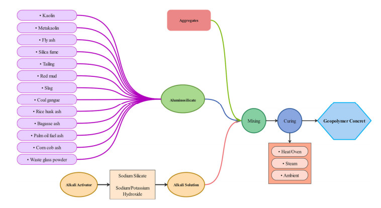
The green concretes industry benefits from utilizing gel to replace parts of the cement in concretes. However, measuring the compressive strength of geo-polymer concretes (CSGPoC) needs a significant amount of work and expenditure. Therefore, the best idea is predicting CSGPoC with a high level of accuracy. To do this, the base learner and super learner machine learning models were proposed in this study to anticipate CSGPoC. The decision tree (DT) is applied as base learner, and the random forest and extreme gradient boosting (XGBoost) techniques are used as super learner system. In this regard, a database was provided involving 259 CSGPoC data samples, of which four-fifths of is considered for the training model and one-fifth is selected for the testing models. The values of fly ash, ground-granulated blast-furnace slag (GGBS), Na2SiO3, NaOH, fine aggregate, gravel 4/10 mm, gravel 10/20 mm, water/solids ratio, and NaOH molarity were considered as input of the models to estimate CSGPoC. To evaluate the reliability and performance of the decision tree (DT), XGBoost, and random forest (RF) models, 12 performance evaluation metrics were determined. Based on the obtained results, the highest degree of accuracy is achieved by the XGBoost model with mean absolute error (MAE) of 2.073, mean absolute percentage error (MAPE) of 5.547, Nash–Sutcliffe (NS) of 0.981, correlation coefficient (R) of 0.991, R2 of 0.982, root mean square error (RMSE) of 2.458, Willmott's index (WI) of 0.795, weighted mean absolute percentage error (WMAPE) of 0.046, Bias of 2.073, square index (SI) of 0.054, p of 0.027, mean relative error (MRE) of -0.014, and a20 of 0.983 for the training model and MAE of 2.06, MAPE of 6.553, NS of 0.985, R of 0.993, R2 of 0.986, RMSE of 2.307, WI of 0.818, WMAPE of 0.05, Bias of 2.06, SI of 0.056, p of 0.028, MRE of -0.015, and a20 of 0.949 for the testing model. By importing the testing set into trained models, values of 0.8969, 0.9857, and 0.9424 for R2 were obtained for DT, XGBoost, and RF, respectively, which show the superiority of the XGBoost model in CSGPoC estimation. In conclusion, the XGBoost model is capable of more accurately predicting CSGPoC than DT and RF models.
Citation: Ji Zhou, Zhanlin Su, Shahab Hosseini, Qiong Tian, Yijun Lu, Hao Luo, Xingquan Xu, Chupeng Chen, Jiandong Huang. Decision tree models for the estimation of geo-polymer concrete compressive strength[J]. Mathematical Biosciences and Engineering, 2024, 21(1): 1413-1444. doi: 10.3934/mbe.2024061
The green concretes industry benefits from utilizing gel to replace parts of the cement in concretes. However, measuring the compressive strength of geo-polymer concretes (CSGPoC) needs a significant amount of work and expenditure. Therefore, the best idea is predicting CSGPoC with a high level of accuracy. To do this, the base learner and super learner machine learning models were proposed in this study to anticipate CSGPoC. The decision tree (DT) is applied as base learner, and the random forest and extreme gradient boosting (XGBoost) techniques are used as super learner system. In this regard, a database was provided involving 259 CSGPoC data samples, of which four-fifths of is considered for the training model and one-fifth is selected for the testing models. The values of fly ash, ground-granulated blast-furnace slag (GGBS), Na2SiO3, NaOH, fine aggregate, gravel 4/10 mm, gravel 10/20 mm, water/solids ratio, and NaOH molarity were considered as input of the models to estimate CSGPoC. To evaluate the reliability and performance of the decision tree (DT), XGBoost, and random forest (RF) models, 12 performance evaluation metrics were determined. Based on the obtained results, the highest degree of accuracy is achieved by the XGBoost model with mean absolute error (MAE) of 2.073, mean absolute percentage error (MAPE) of 5.547, Nash–Sutcliffe (NS) of 0.981, correlation coefficient (R) of 0.991, R2 of 0.982, root mean square error (RMSE) of 2.458, Willmott's index (WI) of 0.795, weighted mean absolute percentage error (WMAPE) of 0.046, Bias of 2.073, square index (SI) of 0.054, p of 0.027, mean relative error (MRE) of -0.014, and a20 of 0.983 for the training model and MAE of 2.06, MAPE of 6.553, NS of 0.985, R of 0.993, R2 of 0.986, RMSE of 2.307, WI of 0.818, WMAPE of 0.05, Bias of 2.06, SI of 0.056, p of 0.028, MRE of -0.015, and a20 of 0.949 for the testing model. By importing the testing set into trained models, values of 0.8969, 0.9857, and 0.9424 for R2 were obtained for DT, XGBoost, and RF, respectively, which show the superiority of the XGBoost model in CSGPoC estimation. In conclusion, the XGBoost model is capable of more accurately predicting CSGPoC than DT and RF models.

| [1] |
S. H. Chu, H. Ye, L. Huang, L. G. Li, Carbon fiber reinforced geopolymer (FRG) mix design based on liquid film thickness, Constr. Build. Mater., 269 (2021), 121278. https://doi.org/10.1016/j.conbuildmat.2020.121278 doi: 10.1016/j.conbuildmat.2020.121278

|
| [2] |
J. Huang, M. Zhou, J. Zhang, J. Ren, N. I. Vatin, M. M. S. Sabri, The use of GA and PSO in evaluating the shear strength of steel fiber reinforced concrete beams, KSCE J. Civ. Eng., 26 (2022), 3918–3931. https://doi.org/10.1007/s12205-022-0961-0 doi: 10.1007/s12205-022-0961-0
|
| [3] |
K. V. Teja, P. P. Sai, T. Meena, Investigation on the behaviour of ternary blended concrete with scba and sf, IOP Conf. Ser.: Mater. Sci. Eng., 263 (2017), 032012. https://doi.org/10.1088/1757-899X/263/3/032012 doi: 10.1088/1757-899X/263/3/032012
|
| [4] |
Z. Bayasi, J. Zhou, Properties of silica fume concrete and mortar, Int. Concr. Abstr. Portal, 90 (1993), 349–356. https://doi.org/10.14359/3892 doi: 10.14359/3892
|
| [5] |
X. Li, D. Qin, Y. Hu, W. Ahmad, A. Ahmad, F. Aslam, et al., A systematic review of waste materials in cement-based composites for construction applications, J. Build. Eng., 45 (2022), 103447. https://doi.org/10.1016/j.jobe.2021.103447 doi: 10.1016/j.jobe.2021.103447
|
| [6] |
J. Huang, M. Zhou, J. Zhang, J. Ren, N. I. Vatin, M. M. S. Sabri, Development of a new stacking model to evaluate the strength parameters of concrete samples in laboratory, Iran. J. Sci. Technol. Trans. Civ. Eng., 46 (2022), 4355–4370. https://doi.org/10.1007/s40996-022-00912-y doi: 10.1007/s40996-022-00912-y
|
| [7] | A. Cleetus, R. Shibu, P. M. Sreehari, V. K. Paul, B. Jacob, Analysis and study of the effect of GGBFS on concrete structures, Int. Res. J. Eng. Technol., 5 (2018), 3033–3037. |
| [8] |
Y. Qiu, J. Zhou, Short-term rockburst damage assessment in burst-prone mines: an explainable XGBOOST hybrid model with SCSO algorithm, Rock Mech. Rock Eng., 56 (2023), 8745–8770. https://doi.org/10.1007/s00603-023-03522-w doi: 10.1007/s00603-023-03522-w
|
| [9] |
V. K. Nagaraj, D. L. V. Babu, Assessing the performance of molarity and alkaline activator ratio on engineering properties of self-compacting alkaline activated concrete at ambient temperature, J. Build. Eng., 20 (2018), 137–155. https://doi.org/10.1016/j.jobe.2018.07.005 doi: 10.1016/j.jobe.2018.07.005
|
| [10] |
W. P. Zakka, N. H. A. S. Lim, M. C. Khun, A scientometric review of geopolymer concrete, J. Cleaner Prod., 280 (2021), 124353. https://doi.org/10.1016/j.jclepro.2020.124353 doi: 10.1016/j.jclepro.2020.124353
|
| [11] |
P. Zhang, K. Wang, Q. Li, J. Wang, Y. Ling, Fabrication and engineering properties of concretes based on geopolymers/alkali-activated binders–––a review, J. Cleaner Prod., 258 (2020), 120896. https://doi.org/10.1016/j.jclepro.2020.120896 doi: 10.1016/j.jclepro.2020.120896
|
| [12] |
A. Ahmad, W. Ahmad, F. Aslam, P. Joyklad, Compressive strength prediction of fly ash-based geopolymer concrete via advanced machine learning techniques, Case Stud. Constr. Mater., 16 (2022), e00840. https://doi.org/10.1016/j.cscm.2021.e00840 doi: 10.1016/j.cscm.2021.e00840
|
| [13] |
Y. Qiu, J. Zhou, Short-term rockburst prediction in underground project: insights from an explainable and interpretable ensemble learning model, Acta Geotech., 18 (2023), 6655–6685. https://doi.org/10.1007/s11440-023-01988-0 doi: 10.1007/s11440-023-01988-0
|
| [14] |
F. Farooq, X. Jin, M. F. Javed, A. Akbar, M. I. Shah, F. Aslam, et al., Geopolymer concrete as sustainable material: a state of the art review, Constr. Build. Mater., 306 (2021), 124762. https://doi.org/10.1016/j.conbuildmat.2021.124762 doi: 10.1016/j.conbuildmat.2021.124762
|
| [15] |
A. Hosan, S. Haque, F. Shaikh, Compressive behaviour of sodium and potassium activators synthetized fly ash geopolymer at elevated temperatures: a comparative study, J. Build. Eng., 8 (2016), 123–130. https://doi.org/10.1016/j.jobe.2016.10.005 doi: 10.1016/j.jobe.2016.10.005
|
| [16] |
H. L. Muttashar, M. A. M. Ariffin, M. N. Hussein, M. W. Hussin, S. B. Ishaq, Self-compacting geopolymer concrete with spend garnet as sand replacement, J. Build. Eng., 15 (2018), 85–94. https://doi.org/10.1016/j.jobe.2017.10.007 doi: 10.1016/j.jobe.2017.10.007
|
| [17] |
K. Z. Farhan, M. A. M. Johari, R. Demirboğa, Assessment of important parameters involved in the synthesis of geopolymer composites: a review, Constr. Build. Mater., 264 (2020), 120276. https://doi.org/10.1016/j.conbuildmat.2020.120276 doi: 10.1016/j.conbuildmat.2020.120276
|
| [18] |
C. Herath, C. Gunasekara, D. W. Law, S. Setunge, Long term mechanical performance of nano-engineered high volume fly ash concrete, J. Build. Eng., 43 (2021), 103168. https://doi.org/10.1016/j.jobe.2021.103168 doi: 10.1016/j.jobe.2021.103168
|
| [19] |
W. Ahmad, A. Ahmad, K. A. Ostrowski, F. Aslam, P. Joyklad, P. Zajdel, Application of advanced machine learning approaches to predict the compressive strength of concrete containing supplementary cementitious materials, Materials, 14 (2021), 5762. https://doi.org/10.3390/ma14195762 doi: 10.3390/ma14195762
|
| [20] |
H. K. Tchakouté, C. H. Rüscher, S. Kong, N. Ranjbar, Synthesis of sodium waterglass from white rice husk ash as an activator to produce metakaolin-based geopolymer cements, J. Build. Eng., 6 (2016), 252–261. https://doi.org/10.1016/j.jobe.2016.04.007 doi: 10.1016/j.jobe.2016.04.007
|
| [21] |
A. Ahmad, W. Ahmad, K. Chaiyasarn, K. A. Ostrowski, F. Aslam, P. Zajdel, et al., Prediction of geopolymer concrete compressive strength using novel machine learning algorithms, Polymers, 13 (2021), 3389. https://doi.org/10.3390/polym13193389 doi: 10.3390/polym13193389
|
| [22] |
B. B. Jindal, Investigations on the properties of geopolymer mortar and concrete with mineral admixtures: a review, Constr. Build. Mater., 227 (2019), 116644. https://doi.org/10.1016/j.conbuildmat.2019.08.025 doi: 10.1016/j.conbuildmat.2019.08.025
|
| [23] |
M. S. Reddy, P. Dinakar, B. H. Rao, Mix design development of fly ash and ground granulated blast furnace slag based geopolymer concrete, J. Build. Eng., 20 (2018), 712–722. https://doi.org/10.1016/j.jobe.2018.09.010 doi: 10.1016/j.jobe.2018.09.010
|
| [24] |
J. Zhou, X. Shen, Y. Qiu, X. Shi, K. Du, Microseismic location in hardrock metal mines by machine learning models based on hyperparameter optimization using bayesian optimizer, Rock Mech. Rock Eng., 56 (2023), 8771–8788. https://doi.org/10.1007/s00603-023-03483-0 doi: 10.1007/s00603-023-03483-0
|
| [25] |
C. L. Wong, K. H. Mo, U. J. Alengaram, S. P. Yap, Mechanical strength and permeation properties of high calcium fly ash-based geopolymer containing recycled brick powder, J. Build. Eng., 32 (2020), 101655. https://doi.org/10.1016/j.jobe.2020.101655 doi: 10.1016/j.jobe.2020.101655
|
| [26] |
S. K. John, Y. Nadir, K. Girija, Effect of source materials, additives on the mechanical properties and durability of fly ash and fly ash-slag geopolymer mortar: a review, Constr. Build. Mater., 280 (2021), 122443. https://doi.org/10.1016/j.conbuildmat.2021.122443 doi: 10.1016/j.conbuildmat.2021.122443
|
| [27] |
Y. Zou, C. Zheng, A. Alzahrani, W. Ahmad, A. Ahmad, A. Mohamed, et al., Evaluation of artificial intelligence methods to estimate the compressive strength of geopolymers, Gels, 8 (2022), 271. https://doi.org/10.3390/gels8050271 doi: 10.3390/gels8050271
|
| [28] |
J. Huang, M. Zhou, H. Yuan, M. M. S. Sabri, X. Li, Prediction of the compressive strength for cement-based materials with metakaolin based on the hybrid machine learning method, Materials, 15 (2022), 3500. https://doi.org/10.3390/ma15103500 doi: 10.3390/ma15103500
|
| [29] |
B. Indraratna, D. J. Armaghani, A. G. Correia, H. Hunt, T. Ngo, Prediction of resilient modulus of ballast under cyclic loading using machine learning techniques, Transp. Geotech., 38 (2023), 100895. https://doi.org/10.1016/j.trgeo.2022.100895 doi: 10.1016/j.trgeo.2022.100895
|
| [30] |
S. Medawela, D. J. Armaghani, B. Indraratna, R. K. Rowe, N. Thamwattana, Development of an advanced machine learning model to predict the pH of groundwater in permeable reactive barriers (PRBs) located in acidic terrain, Comput. Geotech., 161 (2023), 105557. https://doi.org/10.1016/j.compgeo.2023.105557 doi: 10.1016/j.compgeo.2023.105557
|
| [31] |
D. J. Armaghani, P. G. Asteris, A comparative study of ANN and ANFIS models for the prediction of cement-based mortar materials compressive strength, Neural Comput. Appl., 33 (2021), 4501–4532. https://doi.org/10.1007/s00521-020-05244-4 doi: 10.1007/s00521-020-05244-4
|
| [32] |
A. D. Skentou, A. Bardhan, A. Mamou, M. E. Lemonis, G. Kumar, P. Samui, et al., Closed-form equation for estimating unconfined compressive strength of granite from three non-destructive tests using soft computing models, Rock Mech. Rock Eng., 56 (2023), 487–514. https://doi.org/10.1007/s00603-022-03046-9 doi: 10.1007/s00603-022-03046-9
|
| [33] |
W. Mahmood, A. S. Mohammed, P. G. Asteris, R. Kurda, D. J. Armaghani, Modeling flexural and compressive strengths behaviour of cement-grouted sands modified with water reducer polymer, Appl. Sci., 12 (2022), 1016. https://doi.org/10.3390/app12031016 doi: 10.3390/app12031016
|
| [34] |
P. G. Asteris, P. B. Lourenço, P. C. Roussis, C. E. Adami, D. J. Armaghani, L. Cavaleri, et al., Revealing the nature of metakaolin-based concrete materials using artificial intelligence techniques, Constr. Build. Mater., 322 (2022), 126500. https://doi.org/10.1016/j.conbuildmat.2022.126500 doi: 10.1016/j.conbuildmat.2022.126500
|
| [35] |
M. S. Barkhordari, D. J. Armaghani, P. G. Asteris, Structural damage identification using ensemble deep convolutional neural network models, CMES-Comp. Model. Eng. Sci., 134 (2023), 835–855. https://doi.org/10.32604/cmes.2022.020840 doi: 10.32604/cmes.2022.020840
|
| [36] |
L. Cavaleri, M. S. Barkhordari, C. C. Repapis, D. J. Armaghani, D. V. Ulrikh, P. G. Asteris, Convolution-based ensemble learning algorithms to estimate the bond strength of the corroded reinforced concrete, Constr. Build. Mater., 359 (2022), 129504. https://doi.org/10.1016/j.conbuildmat.2022.129504 doi: 10.1016/j.conbuildmat.2022.129504
|
| [37] |
M. Koopialipoor, P. G. Asteris, A. S. Mohammed, D. E. Alexakis, A. Mamou, D. J. Armaghani, Introducing stacking machine learning approaches for the prediction of rock deformation, Transp. Geotech., 34 (2022), 100756. https://doi.org/10.1016/j.trgeo.2022.100756 doi: 10.1016/j.trgeo.2022.100756
|
| [38] |
M. Parsajoo, D. J. Armaghani, A. S. Mohammed, M. Khari, S. Jahandari, Tensile strength prediction of rock material using non-destructive tests: a comparative intelligent study, Transp. Geotech., 31 (2021), 100652. https://doi.org/10.1016/j.trgeo.2021.100652 doi: 10.1016/j.trgeo.2021.100652
|
| [39] | D. J. Armaghani, Y. Y. Ming, A. S. Mohammed, E. Momeni, H. Maizir, Effect of SVM kernel functions on bearing capacity assessment of deep foundations, J. Soft Comput. Civ. Eng., 7 (2023), 111–128. Available from: https://www.jsoftcivil.com/article_169219.html. |
| [40] |
E. Momeni, B. He, Y. Abdi, D. J. Armaghani, Novel hybrid XGBoost model to forecast soil shear strength based on some soil index tests, CMES-Comp. Model. Eng. Sci., 136 (2023), 2527–2550. https://doi.org/10.32604/cmes.2023.026531 doi: 10.32604/cmes.2023.026531
|
| [41] |
J. Zhou, Z. Wang, C. Li, W. Wei, S. Wang, D. J. Armaghani, et al., Hybridized random forest with population-based optimization for predicting shear properties of rock fractures, J. Comput. Sci., 72 (2023), 102097. https://doi.org/10.1016/j.jocs.2023.102097 doi: 10.1016/j.jocs.2023.102097
|
| [42] |
J. Huang, M. Zhou, H. Yuan, M. M. Sabri, X. Li, Towards sustainable construction materials: a comparative study of prediction models for green concrete with metakaolin, Buildings, 12 (2022), 772. https://doi.org/10.3390/buildings12060772 doi: 10.3390/buildings12060772
|
| [43] |
A. Ahmad, K. Chaiyasarn, F. Farooq, W. Ahmad, S. Suparp, F. Aslam, Compressive strength prediction via gene expression programming (Gep) and artificial neural network (ann) for concrete containing rca, Buildings, 11 (2021), 324. https://doi.org/10.3390/buildings11080324 doi: 10.3390/buildings11080324
|
| [44] |
H. Song, A. Ahmad, K. A. Ostrowski, M. Dudek, Analyzing the compressive strength of ceramic waste-based concrete using experiment and artificial neural network (Ann) approach, Materials, 14 (2021), 4518. https://doi.org/10.3390/ma14164518 doi: 10.3390/ma14164518
|
| [45] |
H. Nguyen, T. Vu, T. P. Vo, H. T. Thai, Efficient machine learning models for prediction of concrete strengths, Constr. Build. Mater., 266 (2021), 120950. https://doi.org/10.1016/j.conbuildmat.2020.120950 doi: 10.1016/j.conbuildmat.2020.120950
|
| [46] |
J. Huang, Y. Sun, J. Zhang, Reduction of computational error by optimizing SVR kernel coefficients to simulate concrete compressive strength through the use of a human learning optimization algorithm, Eng. Comput., 38 (2022), 3151–3168. https://doi.org/10.1007/s00366-021-01305-x doi: 10.1007/s00366-021-01305-x
|
| [47] |
P. Sarir, J. Chen, P. G. Asteris, D. J. Armaghani, M. M. Tahir, Developing GEP tree-based, neuro-swarm, and whale optimization models for evaluation of bearing capacity of concrete-filled steel tube columns, Eng. Comput., 37 (2021), 1–19. https://doi.org/10.1007/s00366-019-00808-y doi: 10.1007/s00366-019-00808-y
|
| [48] |
F. R. Balf, H. M. Kordkheili, A. M. Kordkheili, A new method for predicting the ingredients of self-compacting concrete (SCC) including fly ash (FA) using data envelopment analysis (DEA), Arabian J. Sci. Eng., 46 (2021), 4439–4460. https://doi.org/10.1007/s13369-020-04927-3 doi: 10.1007/s13369-020-04927-3
|
| [49] |
A. Ahmad, F. Farooq, K. A. Ostrowski, K. Śliwa-Wieczorek, S. Czarnecki, Application of novel machine learning techniques for predicting the surface chloride concentration in concrete containing waste material, Materials, 14 (2021), 2297. https://doi.org/10.3390/ma14092297 doi: 10.3390/ma14092297
|
| [50] |
M. Azimi-Pour, H. Eskandari-Naddaf, A. Pakzad, Linear and non-linear SVM prediction for fresh properties and compressive strength of high volume fly ash self-compacting concrete, Constr. Build. Mater., 230 (2020), 117021. https://doi.org/10.1016/j.conbuildmat.2019.117021 doi: 10.1016/j.conbuildmat.2019.117021
|
| [51] |
P. Saha, P. Debnath, P. Thomas, Prediction of fresh and hardened properties of self-compacting concrete using support vector regression approach, Neural Comput. Appl., 32 (2020), 7995–8010. https://doi.org/10.1007/s00521-019-04267-w doi: 10.1007/s00521-019-04267-w
|
| [52] |
A. A. Shahmansouri, H. A. Bengar, E. Jahani, Predicting compressive strength and electrical resistivity of eco-friendly concrete containing natural zeolite via GEP algorithm, Constr. Build. Mater., 229 (2019), 116883. https://doi.org/10.1016/j.conbuildmat.2019.116883 doi: 10.1016/j.conbuildmat.2019.116883
|
| [53] |
J. Huang, M. M. Sabri, D. V. Ulrikh, M. Ahmad, K. A. Alsaffar, Predicting the compressive strength of the cement-fly ash–slag ternary concrete using the firefly algorithm (FA) and random forest (RF) hybrid machine-learning method, Materials, 15 (2022), 4193. https://doi.org/10.3390/ma15124193 doi: 10.3390/ma15124193
|
| [54] |
F. Aslam, F. Farooq, M. N. Amin, K. Khan, A. Waheed, A. Akbar, et al., Applications of gene expression programming for estimating compressive strength of high-strength concrete, Adv. Civ. Eng., 2020 (2020), 8850535. https://doi.org/10.1155/2020/8850535 doi: 10.1155/2020/8850535
|
| [55] |
F. Farooq, M. N. Amin, K. Khan, M. R. Sadiq, M. F. Javed, F. Aslam, et al., A comparative study of random forest and genetic engineering programming for the prediction of compressive strength of high strength concrete (HSC), Appl. Sci., 10 (2020), 7330. https://doi.org/10.3390/app10207330 doi: 10.3390/app10207330
|
| [56] |
P. G. Asteris, K. G. Kolovos, Self-compacting concrete strength prediction using surrogate models, Neural Comput. Appl., 31 (2019), 409–424. https://doi.org/10.1007/s00521-017-3007-7 doi: 10.1007/s00521-017-3007-7
|
| [57] |
S. Selvaraj, S. Sivaraman, Prediction model for optimized self-compacting concrete with fly ash using response surface method based on fuzzy classification, Neural Comput. Appl., 31 (2019), 1365–1373. https://doi.org/10.1007/s00521-018-3575-1 doi: 10.1007/s00521-018-3575-1
|
| [58] |
J. Zhang, G. Ma, Y. Huang, J. Sun, F. Aslani, B. Nener, Modelling uniaxial compressive strength of lightweight self-compacting concrete using random forest regression, Constr. Build. Mater., 210 (2019), 713–719. https://doi.org/10.1016/j.conbuildmat.2019.03.189 doi: 10.1016/j.conbuildmat.2019.03.189
|
| [59] |
A. Kaveh, T. Bakhshpoori, S. M. Hamze-Ziabari, M5' and mars based prediction models for properties of selfcompacting concrete containing fly ash, Period. Polytech., Civ. Eng., 62 (2018), 281–294. https://doi.org/10.3311/PPci.10799 doi: 10.3311/PPci.10799
|
| [60] |
D. Sathyan, K. B. Anand, A. J. Prakash, B. Premjith, Modeling the fresh and hardened stage properties of self-compacting concrete using random kitchen sink algorithm, Int. J. Concr. Struct. Mater., 12 (2018), 24. https://doi.org/10.1186/s40069-018-0246-7 doi: 10.1186/s40069-018-0246-7
|
| [61] |
B. Vakhshouri, S. Nejadi, Prediction of compressive strength of self-compacting concrete by ANFIS models, Neurocomputing, 280 (2018), 13–22. https://doi.org/10.1016/j.neucom.2017.09.099 doi: 10.1016/j.neucom.2017.09.099
|
| [62] |
O. B. Douma, B. Boukhatem, M. Ghrici, A. Tagnit-Hamou, Prediction of properties of self-compacting concrete containing fly ash using artificial neural network, Neural Comput. Appl., 28 (2017), 707–718. https://doi.org/10.1007/s00521-016-2368-7 doi: 10.1007/s00521-016-2368-7
|
| [63] |
M. A. Yaman, M. A. Elaty, M. Taman, Predicting the ingredients of self compacting concrete using artificial neural network, Alexandria Eng. J., 56 (2017), 523–532. https://doi.org/10.1016/j.aej.2017.04.007 doi: 10.1016/j.aej.2017.04.007
|
| [64] |
A. Ahmad, F. Farooq, P. Niewiadomski, K. Ostrowski, A. Akbar, F. Aslam, et al., Prediction of compressive strength of fly ash based concrete using individual and ensemble algorithm, Materials, 14 (2021), 794. https://doi.org/10.3390/ma14040794 doi: 10.3390/ma14040794
|
| [65] |
F. Farooq, W. Ahmed, A. Akbar, F. Aslam, R. Alyousef, Predictive modeling for sustainable high-performance concrete from industrial wastes: a comparison and optimization of models using ensemble learners, J. Cleaner Prod., 292 (2021), 126032. https://doi.org/10.1016/j.jclepro.2021.126032 doi: 10.1016/j.jclepro.2021.126032
|
| [66] | R. Buši, M. Benšić, I. Miličević, K. Strukar, Prediction models for the mechanical properties of self-compacting concrete with recycled rubber and silica fume, 13 (2020), 1821. https://doi.org/10.3390/ma13081821 |
| [67] |
M. F. Javed, F. Farooq, S. A. Memon, A. Akbar, M. A. Khan, F. Aslam, et al., New prediction model for the ultimate axial capacity of concrete-filled steel tubes: an evolutionary approach, Crystals, 10 (2020), 741. https://doi.org/10.3390/cryst10090741 doi: 10.3390/cryst10090741
|
| [68] |
M. Nematzadeh, A. A. Shahmansouri, M. Fakoor, Post-fire compressive strength of recycled PET aggregate concrete reinforced with steel fibers : optimization and prediction via RSM and GEP, Constr. Build. Mater., 252 (2020), 119057. https://doi.org/10.1016/j.conbuildmat.2020.119057 doi: 10.1016/j.conbuildmat.2020.119057
|
| [69] |
K. Güçlüer, A. Özbeyaz, S. Göymen, O. Günaydın, A comparative investigation using machine learning methods for concrete compressive strength estimation, Mater. Today Commun., 27 (2021), 102278. https://doi.org/10.1016/j.mtcomm.2021.102278 doi: 10.1016/j.mtcomm.2021.102278
|
| [70] |
A. Ahmad, K. A. Ostrowski, M. Maślak, F. Farooq, I. Mehmood, A. Nafees, Comparative study of supervised machine learning algorithms for predicting the compressive strength of concrete at high temperature, Materials, 14 (2021), 4222. https://doi.org/10.3390/ma14154222 doi: 10.3390/ma14154222
|
| [71] |
P. G. Asteris, A. D. Skentou, A. Bardhan, P. Samui, K. Pilakoutas, Predicting concrete compressive strength using hybrid ensembling of surrogate machine learning models, Cem. Concr. Res., 145 (2021), 106449. https://doi.org/10.1016/j.cemconres.2021.106449 doi: 10.1016/j.cemconres.2021.106449
|
| [72] |
W. Emad, A. S. Mohammed, R. Kurda, K. Ghafor, L. Cavaleri, S. M. A. Qaidi, et al., Prediction of concrete materials compressive strength using surrogate models, Structures, 46 (2022), 1243–1267. https://doi.org/10.1016/j.istruc.2022.11.002 doi: 10.1016/j.istruc.2022.11.002
|
| [73] |
Z. Shen, A. F. Deifalla, P. Kamiński, A. Dyczko, Compressive strength evaluation of ultra-high-strength concrete by machine learning, Materials, 15 (2022), 3523. https://doi.org/10.3390/ma15103523 doi: 10.3390/ma15103523
|
| [74] |
A. Kumar, H. C. Arora, N. R. Kapoor, M. A. Mohammed, K. Kumar, A. Majumdar, et al., Compressive strength prediction of lightweight concrete: machine learning models, Sustainability, 14 (2022), 2404. https://doi.org/10.3390/su14042404 doi: 10.3390/su14042404
|
| [75] |
D. K. I. Jaf, P. I. Abdulrahman, A. S. Mohammed, R. Kurda, S. M. A. Qaidi, P. G. Asteris, Machine learning techniques and multi-scale models to evaluate the impact of silicon dioxide (SiO2) and calcium oxide (CaO) in fly ash on the compressive strength of green concrete, Constr. Build. Mater., 400 (2023), 132604. https://doi.org/10.1016/j.conbuildmat.2023.132604 doi: 10.1016/j.conbuildmat.2023.132604
|
| [76] |
W. Mahmood, A. S. Mohammed, P. G. Asteris, H. Ahmed, Soft computing technics to predict the early-age compressive strength of flowable ordinary Portland cement, Soft Comput., 27 (2023), 3133–3150. https://doi.org/10.1007/s00500-022-07505-x doi: 10.1007/s00500-022-07505-x
|
| [77] |
R. Ali, M. Muayad, A. S. Mohammed, P. G. Asteris, Analysis and prediction of the effect of Nanosilica on the compressive strength of concrete with different mix proportions and specimen sizes using various numerical approaches, Struct. Concr., 24 (2023), 4161–4184. https://doi.org/10.1002/suco.202200718 doi: 10.1002/suco.202200718
|
| [78] |
J. Huang, J. Zhang, X. Li, Y. Qiao, R. Zhang, G. S. Kumar, Investigating the effects of ensemble and weight optimization approaches on neural networks' performance to estimate the dynamic modulus of asphalt concrete, Road Mater. Pavement Des., 24 (2023), 1939–1959. https://doi.org/10.1080/14680629.2022.2112061 doi: 10.1080/14680629.2022.2112061
|
| [79] |
J. Zhou, S. Huang, Y. Qiu, Optimization of random forest through the use of MVO, GWO and MFO in evaluating the stability of underground entry-type excavations, Tunnelling Underground Space Technol., 124 (2022), 104494. https://doi.org/10.1016/j.tust.2022.104494 doi: 10.1016/j.tust.2022.104494
|
| [80] |
D. V. Dao, S. H. Trinh, H. B. Ly, B. T. Pham, Prediction of compressive strength of geopolymer concrete using entirely steel slag aggregates: novel hybrid artificial intelligence approaches, Appl. Sci., 9 (2019), 1113. https://doi.org/10.3390/app9061113 doi: 10.3390/app9061113
|
| [81] |
Q. A. Wang, J. Zhang, J. Huang, Simulation of the compressive strength of cemented tailing backfill through the use of firefly algorithm and random forest model, Shock Vib., 2021 (2021), 5536998. https://doi.org/10.1155/2021/5536998 doi: 10.1155/2021/5536998
|
| [82] |
X. Liang, X. Yu, G. Ding, Y. Jing, J. Huang, Environmental and mechanical effects of rubberised open-graded asphalt mixtures incorporating with titanium dioxide: a laboratory investigation, Int. J. Pavement Eng., 24 (2023), 2241604. https://doi.org/10.1080/10298436.2023.2241604 doi: 10.1080/10298436.2023.2241604
|
| [83] |
X. Liang, X. Yu, B. Xu, C. Chen, G. Ding, Y. Jin, et al., Storage stability and compatibility in foamed warm-mix asphalt (FWMA) containing recycled asphalt pavement (RAP) binder, J. Mater. Civ. Eng., 2024. https://doi.org/10.1061/JMCEE7/MTENG-16468 doi: 10.1061/JMCEE7/MTENG-16468
|
| [84] |
G. Gu, F. Xu, X. Huang, S. Ruan, C. Peng, J. Lin, Foamed geopolymer: the relationship between rheological properties of geopolymer paste and pore-formation mechanism, J. Cleaner Prod., 277 (2020), 123238. https://doi.org/10.1016/j.jclepro.2020.123238 doi: 10.1016/j.jclepro.2020.123238
|
| [85] |
J. Huang, J. Xue, Optimization of SVR functions for flyrock evaluation in mine blasting operations, Environ. Earth Sci., 81 (2022), 434. https://doi.org/10.1007/s12665-022-10523-5 doi: 10.1007/s12665-022-10523-5
|
| [86] |
J. Huang, J. Zhang, Y. Gao, H. Liu, Intelligently predict the rock joint shear strength using the support vector regression and firefly algorithm, Lithosphere, 2021 (2021), 2467126. https://doi.org/10.2113/2021/2467126 doi: 10.2113/2021/2467126
|
| [87] |
J. Zhou, X. Shen, Y. Qiu, X. Shi, M. Khandelwal, Cross-correlation stacking-based microseismic source location using three metaheuristic optimization algorithms, Tunnelling Underground Space Technol., 126 (2022), 104570. https://doi.org/10.1016/j.tust.2022.104570 doi: 10.1016/j.tust.2022.104570
|
| [88] |
X. Wang, S. Hosseini, D. J. Armaghani, E. T. Mohamad, Data-driven optimized artificial neural network technique for prediction of flyrock induced by boulder blasting, Mathematics, 11 (2023), 2358. https://doi.org/10.3390/math11102358 doi: 10.3390/math11102358
|
| [89] |
S. Hosseini, R. Poormirzaee, M. Hajihassani, Application of reliability-based back-propagation causality-weighted neural networks to estimate air-overpressure due to mine blasting, Eng. Appl. Artif. Intell., 115 (2022), 105281. https://doi.org/10.1016/j.engappai.2022.105281 doi: 10.1016/j.engappai.2022.105281
|
| [90] |
S. Hosseini, R. Pourmirzaee, D. J. Armaghani, M. M. S. Sabri, Prediction of ground vibration due to mine blasting in a surface lead–zinc mine using machine learning ensemble techniques, Sci. Rep., 13 (2023), 6591. https://doi.org/10.1038/s41598-023-33796-7 doi: 10.1038/s41598-023-33796-7
|
| [91] |
S. Hosseini, M. Monjezi, E. Bakhtavar, A. Mousavi, Prediction of dust emission due to open pit mine blasting using a hybrid artificial neural network, Nat. Resour. Res., 30 (2021), 4773–4788. https://doi.org/10.1007/s11053-021-09930-5 doi: 10.1007/s11053-021-09930-5
|
| [92] |
S. Hosseini, A. Mousavi, M. Monjezi, Prediction of blast-induced dust emissions in surface mines using integration of dimensional analysis and multivariate regression analysis, Arabian J. Geosci., 15 (2022), 163. https://doi.org/10.1007/s12517-021-09376-2 doi: 10.1007/s12517-021-09376-2
|
| [93] |
H. I. Erdal, Two-level and hybrid ensembles of decision trees for high performance concrete compressive strength prediction, Eng. Appl. Artif. Intell., 26 (2013), 1689–1697. https://doi.org/10.1016/j.engappai.2013.03.014 doi: 10.1016/j.engappai.2013.03.014
|
| [94] |
W. B. Chaabene, M. Flah, M. L. Nehdi, Machine learning prediction of mechanical properties of concrete: critical review, Constr. Build. Mater., 260 (2020), 119889. https://doi.org/10.1016/j.conbuildmat.2020.119889 doi: 10.1016/j.conbuildmat.2020.119889
|
| [95] |
L. Breiman, Random forests, Mach. Learn., 45 (2001), 5–32. https://doi.org/10.1023/A:1010933404324 doi: 10.1023/A:1010933404324
|
| [96] | A. Liaw, M. Wiener, Classification and regression by randomForest, R News, 2 (2002), 18–22. |
| [97] | T. Chen, C. Guestrin, XGBoost: a scalable tree boosting system, in Proceedings of the 22nd ACM SIGKDD International Conference on Knowledge Discovery and Data Mining, (2016), 785–794. https://doi.org/10.1145/2939672.2939785 |
| [98] |
J. Zhao, S. Hosseini, Q. Chen, D. J. Armaghani, Super learner ensemble model: a novel approach for predicting monthly copper price in future, Resour. Policy, 85 (2023), 103903. https://doi.org/10.1016/j.resourpol.2023.103903 doi: 10.1016/j.resourpol.2023.103903
|
| [99] |
Q. Wang, J. Qi, S. Hosseini, H. Rasekh, J. Huang, ICA-LightGBM algorithm for predicting compressive strength of geo-polymer concrete, Buildings, 13 (2023), 2278. https://doi.org/10.3390/buildings13092278 doi: 10.3390/buildings13092278
|
| [100] |
E. Bakhtavar, S. Hosseini, K. Hewage, R. Sadiq, Green blasting policy: simultaneous forecast of vertical and horizontal distribution of dust emissions using artificial causality-weighted neural network, J. Cleaner Prod., 283 (2021), 124562. https://doi.org/10.1016/j.jclepro.2020.124562 doi: 10.1016/j.jclepro.2020.124562
|
| [101] |
E. Bakhtavar, S. Hosseini, K. Hewage, R. Sadiq, Air pollution risk assessment using a hybrid fuzzy intelligent probability-based approach: mine blasting dust impacts, Nat. Resour. Res., 30 (2021), 2607–2627. https://doi.org/10.1007/s11053-020-09810-4 doi: 10.1007/s11053-020-09810-4
|
| [102] |
S. Hosseini, R. Poormirzaee, M. Hajihassani, R. Kalatehjari, An ANN-Fuzzy cognitive map-based Z-number theory to predict flyrock induced by blasting in open-pit mines, Rock Mech. Rock Eng., 55 (2022), 4373–4390. https://doi.org/10.1007/s00603-022-02866-z doi: 10.1007/s00603-022-02866-z
|
| [103] |
R. Ali, M. Muayad, A. S. Mohammed, P. G. Asteris, Analysis and prediction of the effect of Nanosilica on the compressive strength of concrete with different mix proportions and specimen sizes using various numerical approaches, Struct. Concr., 24 (2022), 4161–4184. https://doi.org/10.1002/suco.202200718 doi: 10.1002/suco.202200718
|
| [104] |
S. Hosseini, A. Mousavi, M. Monjezi, M. Khandelwal, Mine-to-crusher policy: planning of mine blasting patterns for environmentally friendly and optimum fragmentation using Monte Carlo simulation-based multi-objective grey wolf optimization approach, Resour. Policy, 79 (2022), 103087. https://doi.org/10.1016/j.resourpol.2022.103087 doi: 10.1016/j.resourpol.2022.103087
|
| [105] |
S. Hosseini, R. Poormirzaee, M. Hajihassani, An uncertainty hybrid model for risk assessment and prediction of blast-induced rock mass fragmentation, Int. J. Rock Mech. Min. Sci., 160 (2022), 105250. https://doi.org/10.1016/j.ijrmms.2022.105250 doi: 10.1016/j.ijrmms.2022.105250
|
| [106] |
S. Hosseini, J. Khatti, B. O. Taiwo, Y. Fissha, K. S. Grover, H. Ikeda, et al., Assessment of the ground vibration during blasting in mining projects using different computational approaches, Sci. Rep., 13 (2023), 18582. https://doi.org/10.1038/s41598-023-46064-5 doi: 10.1038/s41598-023-46064-5
|
| [107] |
S. Hosseini, S. Javanshir, H. Sabeti, P. Tahmasebizadeh, Mathematical-based gene expression programming (GEP): a novel model to predict zinc separation from a bench-scale bioleaching process, J. Sustainable Metall., 9 (2023), 1601–1619. https://doi.org/10.1007/s40831-023-00751-9 doi: 10.1007/s40831-023-00751-9
|
| [108] |
S. Hosseini, R. Pourmirzaee, Green policy for managing blasting induced dust dispersion in open-pit mines using probability-based deep learning algorithm, Expert Syst. Appl., 240 (2023), 122469. https://doi.org/10.1016/j.eswa.2023.122469 doi: 10.1016/j.eswa.2023.122469
|
| [109] |
A. I. Lawal, S. Hosseini, M. Kim, N. O. Ogunsola, S. Kwon, Prediction of factor of safety of slopes using stochastically modified ANN and classical methods: a rigorous statistical model selection approach, Nat. Hazard., 2023. https://doi.org/10.1007/s11069-023-06275-5 doi: 10.1007/s11069-023-06275-5
|
| [110] |
M. Apostolopoulou, P. G. Asteris, D. J. Armaghani, M. G. Douvika, P. B. Lourenço, L. Cavaleri, et al., Mapping and holistic design of natural hydraulic lime mortars, Cem. Concr. Res., 136 (2020), 106167. https://doi.org/10.1016/j.cemconres.2020.106167 doi: 10.1016/j.cemconres.2020.106167
|
| [111] |
P. G. Asteris, M. Koopialipoor, D. J. Armaghani, E. A. Kotsonis, P. B. Lourenço, Prediction of cement-based mortars compressive strength using machine learning techniques, Neural Comput. Appl., 33 (2021), 13089–13121. https://doi.org/10.1007/s00521-021-06004-8 doi: 10.1007/s00521-021-06004-8
|
| [112] |
S. Hosseini, M. Monjezi, E. Bakhtavar, Minimization of blast-induced dust emission using gene-expression programming and grasshopper optimization algorithm: a smart mining solution based on blasting plan optimization, Clean Technol. Environ. Policy, 24 (2022), 2313–2328. https://doi.org/10.1007/s10098-022-02327-9 doi: 10.1007/s10098-022-02327-9
|
| [113] |
Y. H. Jong, C. I. Lee, Influence of geological conditions on the powder factor for tunnel blasting, Int. J. Rock Mech. Min. Sci., 41 (2004), 533–538. https://doi.org/10.1016/j.ijrmms.2004.03.095 doi: 10.1016/j.ijrmms.2004.03.095
|


Figures(17) / Tables(2)

Ji Zhou, Zhanlin Su, Shahab Hosseini, Qiong Tian, Yijun Lu, Hao Luo, Xingquan Xu, Chupeng Chen, Jiandong Huang. Decision tree models for the estimation of geo-polymer concrete compressive strength[J]. Mathematical Biosciences and Engineering, 2024, 21(1): 1413-1444. doi: 10.3934/mbe.2024061


 DownLoad: