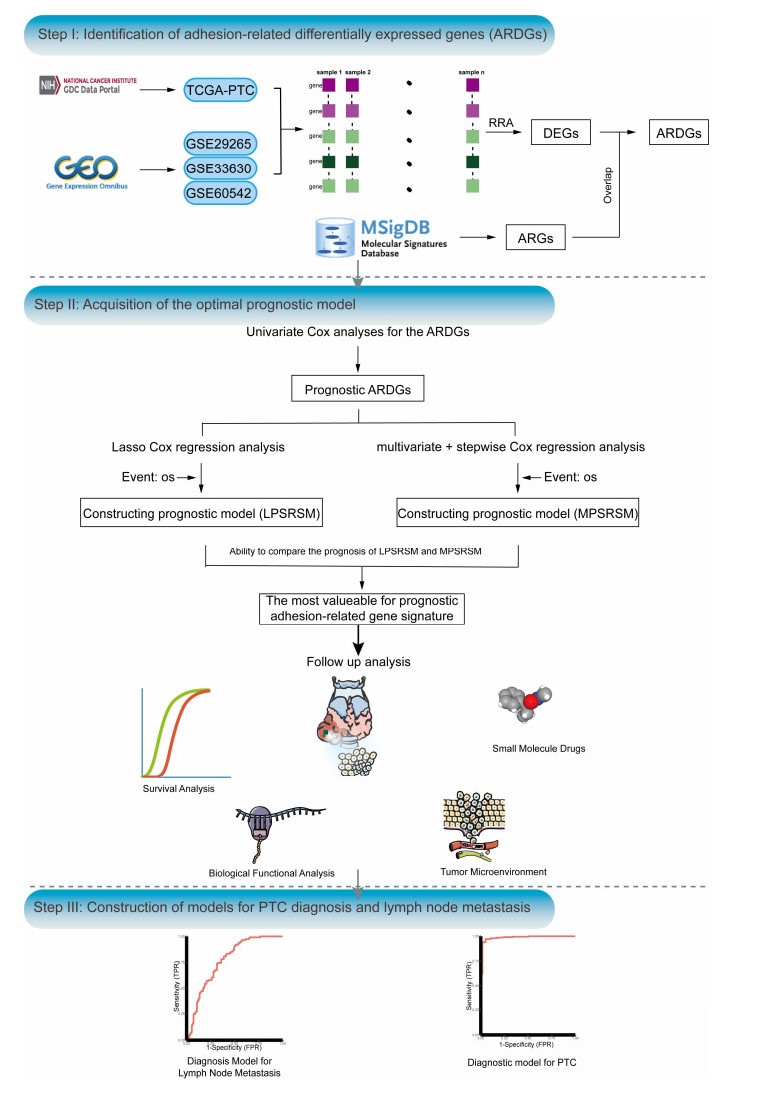
The association between adhesion function and papillary thyroid carcinoma (PTC) is increasingly recognized; however, the precise role of adhesion function in the pathogenesis and prognosis of PTC remains unclear. In this study, we employed the robust rank aggregation algorithm to identify 64 stable adhesion-related differentially expressed genes (ARDGs). Subsequently, using univariate Cox regression analysis, we identified 16 prognostic ARDGs. To construct PTC survival risk scoring models, we employed Lasso Cox and multivariate + stepwise Cox regression methods. Comparative analysis of these models revealed that the Lasso Cox regression model (LPSRSM) displayed superior performance. Further analyses identified age and LPSRSM as independent prognostic factors for PTC. Notably, patients classified as low-risk by LPSRSM exhibited significantly better prognosis, as demonstrated by Kaplan-Meier survival analyses. Additionally, we investigated the potential impact of adhesion feature on energy metabolism and inflammatory responses. Furthermore, leveraging the CMAP database, we screened 10 drugs that may improve prognosis. Finally, using Lasso regression analysis, we identified four genes for a diagnostic model of lymph node metastasis and three genes for a diagnostic model of tumor. These gene models hold promise for prognosis and disease diagnosis in PTC.
Citation: Shuo Sun, Xiaoni Cai, Jinhai Shao, Guimei Zhang, Shan Liu, Hongsheng Wang. Machine learning-based approach for efficient prediction of diagnosis, prognosis and lymph node metastasis of papillary thyroid carcinoma using adhesion signature selection[J]. Mathematical Biosciences and Engineering, 2023, 20(12): 20599-20623. doi: 10.3934/mbe.2023911
The association between adhesion function and papillary thyroid carcinoma (PTC) is increasingly recognized; however, the precise role of adhesion function in the pathogenesis and prognosis of PTC remains unclear. In this study, we employed the robust rank aggregation algorithm to identify 64 stable adhesion-related differentially expressed genes (ARDGs). Subsequently, using univariate Cox regression analysis, we identified 16 prognostic ARDGs. To construct PTC survival risk scoring models, we employed Lasso Cox and multivariate + stepwise Cox regression methods. Comparative analysis of these models revealed that the Lasso Cox regression model (LPSRSM) displayed superior performance. Further analyses identified age and LPSRSM as independent prognostic factors for PTC. Notably, patients classified as low-risk by LPSRSM exhibited significantly better prognosis, as demonstrated by Kaplan-Meier survival analyses. Additionally, we investigated the potential impact of adhesion feature on energy metabolism and inflammatory responses. Furthermore, leveraging the CMAP database, we screened 10 drugs that may improve prognosis. Finally, using Lasso regression analysis, we identified four genes for a diagnostic model of lymph node metastasis and three genes for a diagnostic model of tumor. These gene models hold promise for prognosis and disease diagnosis in PTC.

| [1] |
K. R. Joseph, S. Edirimanne, G. D. Eslick, Multifocality as a prognostic factor in thyroid cancer: A meta-analysis, Int. J. Surg., 50 (2018), 121–125. http://.doi.org/10.1016/j.ijsu.2017.12.035 doi: 10.1016/j.ijsu.2017.12.035

|
| [2] |
A. Arianpoor, M. Asadi, E. Amini, A. Ziaeemehr, Investigating the prevalence of risk factors of papillary thyroid carcinoma recurrence and disease-free survival after thyroidectomy and central neck dissection in Iranian patients, Acta Chir. Belg., 120 (2020), 173–178. http://.doi.org/10.1080/00015458.2019.1576447 doi: 10.1080/00015458.2019.1576447
|
| [3] |
V. Zaydfudim, I. D. Feurer, M. R. Griffin, J. E. Phay, The impact of lymph node involvement on survival in patients with papillary and follicular thyroid carcinoma, Surgery, 144 (2008), 1077–1078. http://.doi.org/10.1016/j.surg.2008.08.034 doi: 10.1016/j.surg.2008.08.034
|
| [4] |
I. M. Boschin, M. R. Pelizzo, F. Giammarile, D. Rubello, P. Colletti, Lymphoscintigraphy in differentiated thyroid cancer, Clin. Nucl. Med., 40 (2015), e343–350. http://.doi.org/10.1097/RLU.0000000000000825 doi: 10.1097/RLU.0000000000000825
|
| [5] |
D. Hou, H. Xu, B. Yuan, J. Liu, Y. Lu, M. Liu, Effects of active localization and vascular preservation of inferior parathyroid glands in central neck dissection for papillary thyroid carcinoma, World J. Surg. Oncol., 18 (2020), 95. http://.doi.org/10.1186/s12957-020-01867-y doi: 10.1186/s12957-020-01867-y
|
| [6] |
I. Elia, G. Doglioni, S. M. Fendt, Metabolic hallmarks of metastasis formation, Trends Cell Biol., 28 (2018), 673–684. http://.doi.org/10.1016/j.tcb.2018.04.002 doi: 10.1016/j.tcb.2018.04.002
|
| [7] |
H. Harjunpää, M. Llort Asens, C. Guenther, S. C. Fagerholm, Cell adhesion molecules and their roles and regulation in the immune and tumor microenvironment, Front. Immunol., 10 (2019), 1078. http://.doi.org/10.3389/fimmu.2019.01078 doi: 10.3389/fimmu.2019.01078
|
| [8] |
L. Mautone, C. Ferravante, A. Tortora, Higher integrin alpha 3 beta1 expression in papillary thyroid cancer is associated with worst outcome, Cancers (Basel), 13 (2021), 2937.http://.doi.org/10.3390/cancers13122937 doi: 10.3390/cancers13122937
|
| [9] | J. Weiss, F. Kuusisto, K. Boyd, Machine learning for treatment assignment: Improving individualized risk attribution, AMIA Annu. Symp. Proc., 2015 (2015), 1306–1315. |
| [10] | J. C. Weiss, D. Page, P. L. Peissig, Statistical Relational Learning to predict primary myocardial infarction from electronic health records, Proc. Innov. Appl. Artif. Intell. Conf., 2012 (2012), 2341–2347. |
| [11] |
M. E. Ritchie, B. Phipson, D. Wu, Limma powers differential expression analyses for RNA-sequencing and microarray studies, Nucleic Acids Res., 43 (2015), e47.http://.doi.org/10.1093/nar/gkv007 doi: 10.1093/nar/gkv007
|
| [12] |
G. Tomas, M. Tarabichi, D. Gacquer, A general method to derive robust organ-specific gene expression-based differentiation indices: application to thyroid cancer diagnostic, Oncogene, 31 (2012), 4490–4498.http://.doi.org/10.1038/onc.2011.626 doi: 10.1038/onc.2011.626
|
| [13] |
M. Tarabichi, M. Saiselet, C. Tresallet, Revisiting the transcriptional analysis of primary tumours and associated nodal metastases with enhanced biological and statistical controls: application to thyroid cancer, Br. J. Cancer, 112 (2015), 1665–1674.http://.doi.org/10.1038/bjc.2014.665 doi: 10.1038/bjc.2014.665
|
| [14] |
A. Subramanian, P. Tamayo, V. K. Mootha, Gene set enrichment analysis: a knowledge-based approach for interpreting genome-wide expression profiles, Proc. Natl. Acad. Sci. U. S. A., 102 (2005), 15545–15550. http://.doi.org/10.1073/pnas.0506580102 doi: 10.1073/pnas.0506580102
|
| [15] |
A. Liberzon, A. Subramanian, R. Pinchback, Molecular signatures database (MSigDB) 3.0, Bioinformatics, 27 (2011), 1739–1740. http://.doi.org/10.1093/bioinformatics/btr260 doi: 10.1093/bioinformatics/btr260
|
| [16] |
A. Liberzon, C. Birger, H. Thorvaldsdottir, The Molecular Signatures Database (MSigDB) hallmark gene set collection, Cell Syst., 1 (2015), 417–425. http://.doi.org/10.1016/j.cels.2015.12.004 doi: 10.1016/j.cels.2015.12.004
|
| [17] |
G. Huang, X. Xu, C. Ju, Identification and validation of autophagy-related gene expression for predicting prognosis in patients with idiopathic pulmonary fibrosis, Front. Immunol., 13 (2022), 997138. http://.doi.org/10.3389/fimmu.2022.997138 doi: 10.3389/fimmu.2022.997138
|
| [18] |
X. Sun, Z. Zhang, Z. Wang, The role of Angiogenesis and remodeling (AR) associated signature for predicting prognosis and clinical outcome of immunotherapy in pan-cancer, Front. Immunol., 13 (2022), 1033967. http://.doi.org/10.3389/fimmu.2022.1033967 doi: 10.3389/fimmu.2022.1033967
|
| [19] |
J. Ruan, S. Xu, R. Chen, EMLI-ICC: an ensemble machine learning-based integration algorithm for metastasis prediction and risk stratification in intrahepatic cholangiocarcinoma, Brief. Bioinform., 23 (2022), bbac450. http://.doi.org/10.1093/bib/bbac450 doi: 10.1093/bib/bbac450
|
| [20] |
X. Wang, L. Yang, C. Yu, An integrated computational strategy to predict personalized cancer drug combinations by reversing drug resistance signatures, Comput. Biol. Med., 163 (2023), 107230. http://.doi.org/10.1016/j.compbiomed.2023.107230 doi: 10.1016/j.compbiomed.2023.107230
|
| [21] |
H. Zhang, P. Xia, J. Liu, ATIC inhibits autophagy in hepatocellular cancer through the AKT/FOXO3 pathway and serves as a prognostic signature for modeling patient survival, Int. J. Biol. Sci., 17 (2021), 4442–4458. http://.doi.org/10.7150/ijbs.65669 doi: 10.7150/ijbs.65669
|
| [22] |
X. Bao, J. Chi, Y. Zhu, High FAAP24 expression reveals poor prognosis and an immunosuppressive microenvironment shaping in AML, Cancer Cell Int., 23 (2023), 117. http://.doi.org/10.1186/s12935-023-02937-3 doi: 10.1186/s12935-023-02937-3
|
| [23] |
B. Cheng, C. Tang, J. Xie, Cuproptosis illustrates tumor micro-environment features and predicts prostate cancer therapeutic sensitivity and prognosis, Life Sci., 325 (2023), 121659. http://.doi.org/10.1016/j.lfs.2023.121659 doi: 10.1016/j.lfs.2023.121659
|
| [24] |
S. He, Y. Ding, Z. Ji, HOPX is a tumor-suppressive biomarker that corresponds to T cell infiltration in skin cutaneous melanoma, Cancer Cell Int., 23 (2023), 122. http://.doi.org/10.1186/s12935-023-02962-2 doi: 10.1186/s12935-023-02962-2
|
| [25] |
Z. Liu, L. Liu, S. Weng, Machine learning-based integration develops an immune-derived lncRNA signature for improving outcomes in colorectal cancer, Nat. Commun., 13 (2022), 816. http://.doi.org/10.1038/s41467-022-28421-6 doi: 10.1038/s41467-022-28421-6
|
| [26] |
Y. Chen, Y. Pan, H. Gao, Mechanistic insights into super-enhancer-driven genes as prognostic signatures in patients with glioblastoma, J. Cancer Res. Clin. Oncol., 149 (2023), 12315–12332. http://.doi.org/10.1007/s00432-023-05121-2 doi: 10.1007/s00432-023-05121-2
|
| [27] |
A. Huang, L. Li, X. Liu, Hedgehog signaling is a potential therapeutic target for vascular calcification, Gene, 872 (2023), 147457. http://.doi.org/10.1016/j.gene.2023.147457 doi: 10.1016/j.gene.2023.147457
|
| [28] |
P. Zhou, J. Shen, X. Ge, Classification and characterisation of extracellular vesicles-related tuberculosis subgroups and immune cell profiles, J. Cell. Mol. Med., 27 (2023), 2482–2494. http://.doi.org/10.1111/jcmm.17836 doi: 10.1111/jcmm.17836
|
| [29] |
R. Kolde, S. Laur, P. Adler, Robust rank aggregation for gene list integration and meta-analysis, Bioinformatics, 28 (2012), 573–580. http://.doi.org/10.1093/bioinformatics/btr709 doi: 10.1093/bioinformatics/btr709
|
| [30] |
C. H. Gao, G. Yu, P. Cai, ggVennDiagram: An intuitive, easy-to-use, and highly customizable R package to generate Venn Diagram, Front. Genet., 12 (2021), 706907. http://.doi.org/10.3389/fgene.2021.706907 doi: 10.3389/fgene.2021.706907
|
| [31] |
Y. Zhou, B. Zhou, L. Pache, Metascape provides a biologist-oriented resource for the analysis of systems-level datasets, Nat. Commun., 10 (2019), 1523. http://.doi.org/10.1038/s41467-019-09234-6 doi: 10.1038/s41467-019-09234-6
|
| [32] |
S. Hanzelmann, R. Castelo, J. Guinney, GSVA: gene set variation analysis for microarray and RNA-seq data, BMC Bioinf., 14 (2013), 7. http://.doi.org/10.1186/1471-2105-14-7 doi: 10.1186/1471-2105-14-7
|
| [33] |
K. Yoshihara, M. Shahmoradgoli, E. Martinez, Inferring tumour purity and stromal and immune cell admixture from expression data, Nat. Commun., 4 (2013), 2612. http://.doi.org/10.1038/ncomms3612 doi: 10.1038/ncomms3612
|
| [34] |
A. M. Newman, C. L. Liu, M. R. Green, Robust enumeration of cell subsets from tissue expression profiles, Nat. Methods, 12 (2015), 453–457. http://.doi.org/10.1038/nmeth.3337 doi: 10.1038/nmeth.3337
|
| [35] |
J. H. Friedman, T. Hastie, R. Tibshirani, Regularization paths for generalized linear models via coordinate descent, J. Stat. Software, 33 (2010), 1–22. http://.doi.org/10.18637/jss.v033.i01 doi: 10.18637/jss.v033.i01
|
| [36] |
P. Blanche, J. F. Dartigues, H. Jacqmin-Gadda, Estimating and comparing time-dependent areas under receiver operating characteristic curves for censored event times with competing risks, Stat. Med., 32 (2013), 5381–5397. http://.doi.org/10.1002/sim.5958 doi: 10.1002/sim.5958
|
| [37] |
M. Kuhn, Building Predictive models in R using the caret package, J. Stat. Software, 28 (2008), 1–26. http://.doi.org/10.18637/jss.v028.i05 doi: 10.18637/jss.v028.i05
|
| [38] |
M. Uhlen, C. Zhang, S. Lee, A pathology atlas of the human cancer transcriptome, Science, 357 (2017), eaan2507. http://.doi.org/10.1126/science.aan2507 doi: 10.1126/science.aan2507
|
| [39] |
N. Enz, G. Vliegen, I. De Meester, CD26/DPP4-a potential biomarker and target for cancer therapy, Pharmacol Ther, 198 (2019), 135–159. http://.doi.org/10.1016/j.pharmthera.2019.02.015 doi: 10.1016/j.pharmthera.2019.02.015
|
| [40] |
Q. He, H. Cao, Y. Zhao, Dipeptidyl peptidase-4 stabilizes integrin alpha4beta1 complex to promote thyroid cancer cell metastasis by activating transforming growth factor-beta signaling pathway, Thyroid, 32 (2022), 1411–1422. http://.doi.org/10.1089/thy.2022.0317 doi: 10.1089/thy.2022.0317
|
| [41] |
X. Hu, S. Chen, C. Xie, DPP4 gene silencing inhibits proliferation and epithelial-mesenchymal transition of papillary thyroid carcinoma cells through suppression of the MAPK pathway, J. Endocrinol. Invest., 44 (2021), 1609–1623. http://.doi.org/10.1007/s40618-020-01455-7 doi: 10.1007/s40618-020-01455-7
|
| [42] |
G. Peppino, R. Ruiu, M. Arigoni, Teneurins: Role in cancer and potential role as diagnostic biomarkers and targets for therapy, Int. J. Mol. Sci., 22 (2021), 2321. http://.doi.org/10.3390/ijms22052321 doi: 10.3390/ijms22052321
|
| [43] |
S. P. Cheng, M. J. Chen, M. N. Chien, Overexpression of teneurin transmembrane protein 1 is a potential marker of disease progression in papillary thyroid carcinoma, Clin. Exper. Med., 17 (2017), 555–564. http://.doi.org/10.1007/s10238-016-0445-y doi: 10.1007/s10238-016-0445-y
|
| [44] |
S. Lemarchant, M. Pruvost, J. Montaner, ADAMTS proteoglycanases in the physiological and pathological central nervous system, J. Neuroinflamm., 10 (2013), 133. http://.doi.org/10.1186/1742-2094-10-133 doi: 10.1186/1742-2094-10-133
|
| [45] |
W. Sun, G. Ma, L. Zhang, DNMT3A-mediated silence in ADAMTS9 expression is restored by RNF180 to inhibit viability and motility in gastric cancer cells, Cell Death Dis., 12 (2021), 428. http://.doi.org/10.1038/s41419-021-03628-5 doi: 10.1038/s41419-021-03628-5
|
| [46] |
N. Wang, X. Huo, B. Zhang, METTL3-Mediated ADAMTS9 Suppression facilitates angiogenesis and carcinogenesis in gastric cancer, Front. Oncol., 12 (2022), 861807. http://.doi.org/10.3389/fonc.2022.861807 doi: 10.3389/fonc.2022.861807
|
| [47] |
K. Goto, M. Morimoto, M. Osaki, The impact of AMIGO2 on prognosis and hepatic metastasis in gastric cancer patients, BMC Cancer, 22 (2022), 280. http://.doi.org/10.1186/s12885-022-09339-0 doi: 10.1186/s12885-022-09339-0
|
| [48] |
R. Izutsu, M. Osaki, J. P. Jehun, Liver metastasis formation is defined by AMIGO2 expression via adhesion to hepatic endothelial cells in human gastric and colorectal cancer cells, Pathol. Res. Pract., 237 (2022), 154015. http://.doi.org/10.1016/j.prp.2022.154015 doi: 10.1016/j.prp.2022.154015
|
| [49] |
Z. Han, Y. Feng, Y. Deng, Integrated analysis reveals prognostic value and progression-related role of AMIGO2 in prostate cancer, Transl. Androl. Urol., 11 (2022), 914–928. http://.doi.org/10.21037/tau-21-1148 doi: 10.21037/tau-21-1148
|
| [50] |
E. Rassart, F. Desmarais, O. Najyb, Apolipoprotein D, Gene, 756 (2020), 144874. http://.doi.org/10.1016/j.gene.2020.144874 doi: 10.1016/j.gene.2020.144874
|
| [51] |
F. Desmarais, V. Herve, K. F. Bergeron, Cerebral apolipoprotein D exits the brain and accumulates in peripheral tissues, Int. J. Mol. Sci., 22 (2021), 4118. http://.doi.org/10.3390/ijms22084118 doi: 10.3390/ijms22084118
|
| [52] |
C. J. Lai, H. C. Cheng, C. Y. Lin, Activation of liver X receptor suppresses angiogenesis via induction of ApoD, Faseb J., 31 (2017), 5568–5576. http://.doi.org/10.1096/fj.201700374R doi: 10.1096/fj.201700374R
|
| [53] |
M. Schulze, C. Violonchi, S. Swoboda, RELN signaling modulates glioblastoma growth and substrate-dependent migration, Brain Pathol., 28 (2018), 695–709. http://.doi.org/10.1111/bpa.12584 doi: 10.1111/bpa.12584
|
| [54] | O. Dohi, H. Takada, N. Wakabayashi, Epigenetic silencing of RELN in gastric cancer, Int. J. Oncol., 36 (2010), 85–92. http://doi.org/10.3892/ijo_00000478 |
| [55] |
Z. Li, X. Wang, Y. Yang, Identification and validation of RELN mutation as a response indicator for immune checkpoint inhibitor therapy in melanoma and non-small cell lung cancer, Cells, 11 (2022), 3841. http://.doi.org/10.3390/cells11233841 doi: 10.3390/cells11233841
|
| [56] |
N. Rufo, A. D. Garg, P. Agostinis, The unfolded protein response in immunogenic cell death and cancer immunotherapy, Trends Cancer, 3 (2017), 643–658. http://.doi.org/10.1016/j.trecan.2017.07.002 doi: 10.1016/j.trecan.2017.07.002
|
| [57] |
R. Saghaleyni, A. Sheikh Muhammad, P. Bangalore, Machine learning-based investigation of the cancer protein secretory pathway, PLoS Comput. Biol., 17 (2021), e1008898. http://.doi.org/10.1371/journal.pcbi.1008898 doi: 10.1371/journal.pcbi.1008898
|
| [58] |
C. T. Walsh, B. P. Tu, Y. Tang, Eight kinetically stable but thermodynamically activated molecules that power cell metabolism, Chem. Rev., 118 (2018), 1460–1494. http://.doi.org/10.1021/acs.chemrev.7b00510 doi: 10.1021/acs.chemrev.7b00510
|
| [59] |
S. Y. Lunt, S. M. Fendt, Metabolism – A cornerstone of cancer initiation, progression, immune evasion and treatment response, Curr. Opin. Syst. Biol., 8 (2018), 67–72. https://doi.org/10.1016/j.coisb.2017.12.006 doi: 10.1016/j.coisb.2017.12.006
|
| [60] |
V. Friand, G. David, P. Zimmermann, Syntenin and syndecan in the biogenesis of exosomes, Biol. Cell., 107 (2015), 331–341. http://.doi.org/10.1111/boc.201500010 doi: 10.1111/boc.201500010
|
| [61] |
S. Y. Lunt, M. G. Vander Heiden, Aerobic glycolysis: meeting the metabolic requirements of cell proliferation, Annu. Rev. Cell Dev. Biol., 27 (2011), 441–464. http://.doi.org/10.1146/annurev-cellbio-092910-154237 doi: 10.1146/annurev-cellbio-092910-154237
|
| [62] |
B. Sousa, J. Pereira, J. Paredes, The crosstalk between cell adhesion and cancer metabolism, Int. J. Mol. Sci., 20 (2019), 1933. http://.doi.org/10.3390/ijms20081933 doi: 10.3390/ijms20081933
|
| [63] |
D. Hanahan, L. M. Coussens, Accessories to the crime: functions of cells recruited to the tumor microenvironment, Cancer Cell, 21 (2012), 309–322. http://.doi.org/10.1016/j.ccr.2012.02.022 doi: 10.1016/j.ccr.2012.02.022
|
 mbe-20-12-911 supplementary.pdf mbe-20-12-911 supplementary.pdf |
 |


Figures(9)

Shuo Sun, Xiaoni Cai, Jinhai Shao, Guimei Zhang, Shan Liu, Hongsheng Wang. Machine learning-based approach for efficient prediction of diagnosis, prognosis and lymph node metastasis of papillary thyroid carcinoma using adhesion signature selection[J]. Mathematical Biosciences and Engineering, 2023, 20(12): 20599-20623. doi: 10.3934/mbe.2023911


 DownLoad: