Climate change and the rapid development of cities have brought considerable challenges to the sustainable development of urban and rural areas, and using nature-based solutions to strengthen ecosystems' resilience and response capacity has become a consensus strategy. Natural solutions are the collective name for all solutions that increase the city's resilience while benefiting the environment and humanity. To deepen the theoretical research and practical development of NBS, I reviewed 87 papers on NBS through the Web of Science database. The study found that NBS-related research mostly focuses on five aspects: Concept of ideas, applied technology, implementation guidelines, performance evaluation and platform building. Currently, the emphasis is predominantly on ideas and platform development in developed countries. While the other three domains were also explored, they primarily adhere to conventional methodologies and content within the NBS context. While NBS research covered many areas and boasts an integrative, collaborative approach, it remained fragmented and lacked a cohesive system. On this basis, I proposed a systematic framework to strengthen the systematicity of the NBS system, give full play to the unique advantages of NBS as a comprehensive concept and promote the specific implementation and development of NBS. I examined NBS's progression and benefits, providing a thorough insight into its significance in sustainable urban development. The research introduced a cohesive framework by elucidating NBS's foundational concepts guiding subsequent inquiries. Such findings are pivotal for facilitating informed strategies and enhancing resilience to climate adversities, underscoring a comprehensive approach to sustainability.
Citation: Hongpeng Fu. A comprehensive review of nature-based solutions: current status and future research[J]. AIMS Environmental Science, 2023, 10(5): 677-690. doi: 10.3934/environsci.2023037
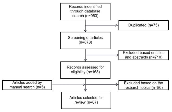
Climate change and the rapid development of cities have brought considerable challenges to the sustainable development of urban and rural areas, and using nature-based solutions to strengthen ecosystems' resilience and response capacity has become a consensus strategy. Natural solutions are the collective name for all solutions that increase the city's resilience while benefiting the environment and humanity. To deepen the theoretical research and practical development of NBS, I reviewed 87 papers on NBS through the Web of Science database. The study found that NBS-related research mostly focuses on five aspects: Concept of ideas, applied technology, implementation guidelines, performance evaluation and platform building. Currently, the emphasis is predominantly on ideas and platform development in developed countries. While the other three domains were also explored, they primarily adhere to conventional methodologies and content within the NBS context. While NBS research covered many areas and boasts an integrative, collaborative approach, it remained fragmented and lacked a cohesive system. On this basis, I proposed a systematic framework to strengthen the systematicity of the NBS system, give full play to the unique advantages of NBS as a comprehensive concept and promote the specific implementation and development of NBS. I examined NBS's progression and benefits, providing a thorough insight into its significance in sustainable urban development. The research introduced a cohesive framework by elucidating NBS's foundational concepts guiding subsequent inquiries. Such findings are pivotal for facilitating informed strategies and enhancing resilience to climate adversities, underscoring a comprehensive approach to sustainability.

| [1] |
Head BW, Xiang WN (2016) Working with wicked problems in socio-ecological systems: More awareness, greater acceptance, and better adaptation. Landsc Urban Plan 154: 1–3. https://doi.org/10.1016/j.landurbplan.2016.07.011 doi: 10.1016/j.landurbplan.2016.07.011

|
| [2] |
Scott M, Lennon M, Haase D, et al. (2016) Nature-based solutions for the contemporary city: insights from practice in Fingal, Ireland. Plan Theory Pract 17: 267–300. https://doi.org/10.1080/14649357.2016.1158907 doi: 10.1080/14649357.2016.1158907
|
| [3] |
Lafortezza R, Chen J, van den Bosch CK, et al. (2018) Nature-based solutions for resilient landscapes and cities. Environ Res 165: 431–441. https://doi.org/10.1016/j.envres.2017.11.038 doi: 10.1016/j.envres.2017.11.038
|
| [4] |
Wang Z, Fu H, Jian Y, et al. (2022) On the comparative use of social media data and survey data in prioritizing ecosystem services for cost-effective governance. Ecosyst Serv 56: 101446. https://doi.org/10.1016/j.ecoser.2022.101446 doi: 10.1016/j.ecoser.2022.101446
|
| [5] |
Cohen-Shacham E, Andrade A, Dalton J, et al. (2019) Core principles for successfully implementing and upscaling Nature-based Solutions. Environ Sci Policy 98: 20–29. https://doi.org/10.1016/j.envsci.2019.04.014 doi: 10.1016/j.envsci.2019.04.014
|
| [6] |
C Mell I (2015) Establishing the rationale for green infrastructure investment in Indian cities: is the mainstreaming of urban greening an expanding or diminishing reality? AIMS Environ Sci 2: 134–153. https://doi.org/10.3934/environsci.2015.2.134 doi: 10.3934/environsci.2015.2.134
|
| [7] | Millennium Ecosystem Assessment (MEA), 2005. Ecosystems and Human Well-being: Synthesis. Island Press, Washington, DC. |
| [8] |
Wang Z, Jie H, Fu H, et al. (2022) A social-media-based improvement index for urban renewal. Ecol Indic 137: 108775. https://doi.org/10.1016/j.ecolind.2022.108775 doi: 10.1016/j.ecolind.2022.108775
|
| [9] |
Russo A, Escobedo FJ, Zerbe S (2016) Quantifying the local-scale ecosystem services provided by urban treed streetscapes in bolzano, italy. AIMS Environ Sci 3: 58–76. https://doi.org/10.3934/environsci.2016.1.58 doi: 10.3934/environsci.2016.1.58
|
| [10] |
Atanasova N, Castellar JAC, Pineda-Martos R, et al. (2021) Nature-Based Solutions and Circularity in Cities. Circ Econ Sustain 1: 319–332. https://doi.org/10.1007/s43615-021-00024-1 doi: 10.1007/s43615-021-00024-1
|
| [11] |
Sgroi F (2021) Landscape management and economic evaluation of the ecosystem services of the vineyards. AIMS Environ Sci 8: 393–402. https://doi.org/10.3934/environsci.2021025 doi: 10.3934/environsci.2021025
|
| [12] |
Jiang Q, Wang Z, Yu K, et al. (2023) The influence of urbanization on local perception of the effect of traditional landscapes on human wellbeing: A case study of a pondscape in Chongqing, China. Ecosyst Serv 60: 101521. https://doi.org/10.1016/j.ecoser.2023.101521 doi: 10.1016/j.ecoser.2023.101521
|
| [13] |
Sarabi SE, Han Q, Romme AGL, et al. (2019) Key enablers of and barriers to the uptake and implementation of nature-based solutions in urban settings: A review. Resources 8. https://doi.org/10.3390/resources8030121 doi: 10.3390/resources8030121
|
| [14] |
Liu Y, Wu YC, Fu H, et al. (2023) Digital intervention in improving the outcomes of mental health among LGBTQ+ youth: a systematic review. Front Psychol 14: 1242928. https://doi.org/10.3389/fpsyg.2023.1242928 doi: 10.3389/fpsyg.2023.1242928
|
| [15] | Fu H, Wang Z, Jie H, et al. (2021) Emotional Characteristics and Influencing Factors of Urban Park Users: A Case Study of South China Botanical Garden and Yuexiu Park. Beijing Daxue Xuebao (Ziran Kexue Ban)/Acta Scientiarum Naturalium Universitatis Pekinensis 57: 1108–1120. |
| [16] |
Seddon N, Chausson A, Berry P, et al. (2020) Understanding the value and limits of nature-based solutions to climate change and other global challenges. Philos Trans R Soc B Biol Sci 375. https://doi.org/10.1098/rstb.2019.0120 doi: 10.1098/rstb.2019.0120
|
| [17] |
Nelson DR, Bledsoe BP, Ferreira S, et al. (2020) Challenges to realizing the potential of nature-based solutions. Curr Opin Environ Sustain 45: 49–55. ttps://doi.org/10.1016/j.cosust.2020.09.001 doi: 10.1016/j.cosust.2020.09.001
|
| [18] | IUCN (2016).The IUCN Programme 2013-2016, Gland (2016), 25-30. |
| [19] |
van den Bosch M, Ode Sang (2017) Urban natural environments as nature-based solutions for improved public health – A systematic review of reviews. Environ Res 158: 373–384. https://doi.org/10.1016/j.envres.2017.05.040 doi: 10.1016/j.envres.2017.05.040
|
| [20] |
Kronenberg J (2015) Betting against Human Ingenuity: The Perils of the Economic Valuation of Nature's Services. Bioscience 65: 1096–1099. https://doi.org/10.1093/biosci/biv135 doi: 10.1093/biosci/biv135
|
| [21] |
McFarland AR, Larsen L, Yeshitela K, et al. (2019). Guide for using green infrastructure in urban environments for stormwater management. Environ Sci Wat Res Technol 5: 643–659. https://doi.org/10.1039/C8EW00498F doi: 10.1039/C8EW00498F
|
| [22] |
Xiang P, Wang Y, Deng Q (2017) Inclusive nature-based solutions for urban regeneration in a natural disaster vulnerability context: A case study of Chongqing, China. Sustainability (Switzerland) 9. https://doi.org/10.3390/su9071205 doi: 10.3390/su9071205
|
| [23] |
Blau ML, Luz F, Panagopoulos T (2018) Urban river recovery inspired by nature-based solutions and biophilic design in Albufeira, Portugal. Land (Basel) 7. https://doi.org/10.3390/land7040141 doi: 10.3390/land7040141
|
| [24] |
Raymond CM, Frantzeskaki N, Kabisch N, et al. (2017) A framework for assessing and implementing the co-benefits of nature-based solutions in urban areas. Environ Sci Policy 77: 15–24. https://doi.org/10.1016/j.envsci.2017.07.008 doi: 10.1016/j.envsci.2017.07.008
|
| [25] |
Frantzeskaki N, McPhearson T, Collier MJ, et al. (2019) Nature-based solutions for urban climate change adaptation: Linking science, policy, and practice communities for evidence-based decision-making. Bioscience 69: 455–466. https://doi.org/10.1093/biosci/biz042 doi: 10.1093/biosci/biz042
|
| [26] |
van der Jagt APN, Szaraz LR, Delshammar T, et al. (2017) Cultivating nature-based solutions: The governance of communal urban gardens in the European Union. Environ Res 159: 264–275. https://doi.org/10.1016/j.envres.2017.08.013 doi: 10.1016/j.envres.2017.08.013
|
| [27] |
Nesshöver C, Assmuth T, Irvine KN, et al. (2017) The science, policy and practice of nature-based solutions: An interdisciplinary perspective. Sci Total Environ 579: 1215–1227. https://doi.org/10.1016/j.scitotenv.2016.11.106 doi: 10.1016/j.scitotenv.2016.11.106
|
| [28] |
Boelee E, Janse J, Le Gal A, et al. (2017) Overcoming water challenges through nature-based solutions. Water Policy 19: 820–836. https://doi.org/10.2166/wp.2017.105 doi: 10.2166/wp.2017.105
|
| [29] |
Faivre N, Fritz M, Freitas T, et al. (2017) Nature-Based Solutions in the EU: Innovating with nature to address social, economic and environmental challenges. Environ Res 159: 509–518. https://doi.org/10.1016/j.envres.2017.08.032 doi: 10.1016/j.envres.2017.08.032
|
| [30] |
Xing Y, Jones P, Donnison I (2017) Characterisation of nature-based solutions for the built environment. Sustainability 9. https://doi.org/10.3390/su9010149 doi: 10.3390/su9010149
|
| [31] |
Panno A, Carrus G, Lafortezza R, et al. (2017) Nature-based solutions to promote human resilience and wellbeing in cities during increasingly hot summers. Environ Res 159: 249–256. https://doi.org/10.1016/j.envres.2017.08.016 doi: 10.1016/j.envres.2017.08.016
|
| [32] |
Cariñanos P, Casares-Porcel M, Díaz de la Guardia C, et al. (2017) Assessing allergenicity in urban parks: A nature-based solution to reduce the impact on public health. Environ Res 155: 219–227. https://doi.org/10.1016/j.envres.2017.02.015 doi: 10.1016/j.envres.2017.02.015
|
| [33] |
Tomao A, Quatrini V, Corona P, et al. (2017) Resilient landscapes in Mediterranean urban areas: Understanding factors influencing forest trends. Environ Res 156: 1–9. https://doi.org/10.1016/j.envres.2017.03.006 doi: 10.1016/j.envres.2017.03.006
|
| [34] |
Lin Z, Qi J (2017) Hydro-dam – A nature-based solution or an ecological problem: The fate of the Tonlé Sap Lake. Environ Res 158: 24–32. https://doi.org/10.1016/j.envres.2017.05.016 doi: 10.1016/j.envres.2017.05.016
|
| [35] |
Chen E, Bridgeman T (2017) The reduction of Chlorella vulgaris concentrations through UV-C radiation treatments: A nature-based solution (NBS). Environ Res 156: 183–189. https://doi.org/10.1016/j.envres.2017.03.007 doi: 10.1016/j.envres.2017.03.007
|
| [36] |
Schaubroeck T (2018) Towards a general sustainability assessment of human/industrial and nature-based solutions. Sustain Sci 13: 1185–1191. https://doi.org/10.1007/s11625-018-0559-0 doi: 10.1007/s11625-018-0559-0
|
| [37] |
Liquete C, Udias A, Conte G, et al. (2016) Integrated valuation of a nature-based solution for water pollution control. Highlighting hidden benefits. Ecosyst Serv 22: 392–401. https://doi.org/10.1016/j.ecoser.2016.09.011 doi: 10.1016/j.ecoser.2016.09.011
|
| [38] |
Wendling LA, Huovila A, zu Castell-Rüdenhausen M, et al. (2018) Benchmarking nature-based solution and smart city assessment schemes against the sustainable development goal indicator framework. Front Environ Sci 6. https://doi.org/10.3389/fenvs.2018.00069 doi: 10.3389/fenvs.2018.00069
|
| [39] |
Calliari E, Staccione A, Mysiak J (2019) An assessment framework for climate-proof nature-based solutions. Sci Total Environ 656: 691–700. https://doi.org/10.1016/j.scitotenv.2018.11.341 doi: 10.1016/j.scitotenv.2018.11.341
|
| [40] |
Mabon L (2019) Enhancing post-disaster resilience by 'building back greener': Evaluating the contribution of nature-based solutions to recovery planning in Futaba County, Fukushima Prefecture, Japan. Landsc Urban Plan 187: 105–118. https://doi.org/10.1016/j.landurbplan.2019.03.013 doi: 10.1016/j.landurbplan.2019.03.013
|
| [41] |
Wild TC, Dempsey N, Broadhead AT (2019) Volunteered information on nature-based solutions — Dredging for data on deculverting. Urban For Urban Green 40: 254–263. https://doi.org/10.1016/j.landurbplan.2019.03.013 doi: 10.1016/j.landurbplan.2019.03.013
|
| [42] |
Santoro S, Pluchinotta I, Pagano A, et al. (2019) Assessing stakeholders' risk perception to promote Nature Based Solutions as flood protection strategies: The case of the Glinščica river (Slovenia). Sci Total Environ 655: 188–201. https://doi.org/10.1016/j.scitotenv.2018.11.116 doi: 10.1016/j.scitotenv.2018.11.116
|
| [43] |
Gulsrud NM, Hertzog K, Shears I (2018) Innovative urban forestry governance in Melbourne?: Investigating "green placemaking" as a nature-based solution. Environ Res 161: 158–167. https://doi.org/10.1016/j.envres.2017.11.005 doi: 10.1016/j.envres.2017.11.005
|


Figures(3) / Tables(2)

Hongpeng Fu. A comprehensive review of nature-based solutions: current status and future research[J]. AIMS Environmental Science, 2023, 10(5): 677-690. doi: 10.3934/environsci.2023037


 DownLoad: