Anther culture is a widely utilized technique in rice breeding because of its simplicity and effectiveness in rapidly obtaining pure lines in the form of doubled haploid plants. The selection of doubled haploid (DH) rice lines derived from anther culture in advanced yield trials is an important step for obtaining superior DH lines. We aimed to determine agronomic performance, including yield and yield stability in order to select lowland DH rice lines that are high yield and have good agronomic performance based on the selection index method. The research was conducted in Indonesia at three locations, i.e., Bogor (West Java), Indramayu (West Java) and Malang (East Java) from July to December 2022. The genotypes tested were 29 DH lines and three check varieties (Inpari-42 Agritan GSR, Inpari-18 Agritan and Bioni63 Ciherang Agritan) using a randomized complete block design (RCBD) with genotypes as a single factor and three replications. High heritability values are found in all agronomic characters, except the percentage of filled grain/panicle, the percentage of empty grain/panicle and productivity. The yield stability based on the Kang method showed that 15 lines were stable and had high productivity. Phenotypic correlation analysis showed that the number of productive tillers, days to flowering, days to harvesting, number of filled grains/panicle and percentage of filled grains all had positive values and significantly correlated with productivity. Phenotypic path analysis showed that the character of days to harvesting, number of filled grains/panicle, number of productive tillers and percentage of filled grains/panicle directly affected the productivity. Based on the weighted selection index, 12 DH lines were selected due to having a positive and higher index (8.54 to 0.28) than the Bioni63 Agritan and Inpari 18 check varieties. Among those lines, 9 DH lines were also stable based on the Kang Method.
Citation: Wira Hadianto, Bambang Sapta Purwoko, Iswari Saraswati Dewi, Willy Bayuardi Suwarno, Purnama Hidayat, Iskandar Lubis. Agronomic performance, yield stability and selection of doubled haploid rice lines in advanced yield trials[J]. AIMS Agriculture and Food, 2023, 8(4): 1010-1027. doi: 10.3934/agrfood.2023054
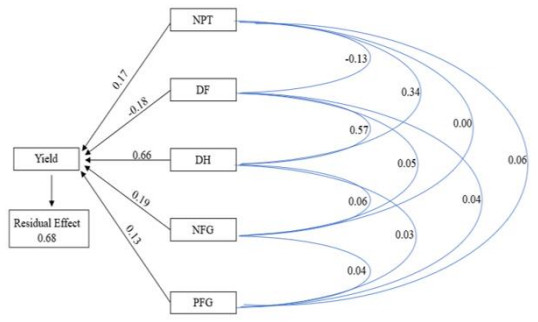
Anther culture is a widely utilized technique in rice breeding because of its simplicity and effectiveness in rapidly obtaining pure lines in the form of doubled haploid plants. The selection of doubled haploid (DH) rice lines derived from anther culture in advanced yield trials is an important step for obtaining superior DH lines. We aimed to determine agronomic performance, including yield and yield stability in order to select lowland DH rice lines that are high yield and have good agronomic performance based on the selection index method. The research was conducted in Indonesia at three locations, i.e., Bogor (West Java), Indramayu (West Java) and Malang (East Java) from July to December 2022. The genotypes tested were 29 DH lines and three check varieties (Inpari-42 Agritan GSR, Inpari-18 Agritan and Bioni63 Ciherang Agritan) using a randomized complete block design (RCBD) with genotypes as a single factor and three replications. High heritability values are found in all agronomic characters, except the percentage of filled grain/panicle, the percentage of empty grain/panicle and productivity. The yield stability based on the Kang method showed that 15 lines were stable and had high productivity. Phenotypic correlation analysis showed that the number of productive tillers, days to flowering, days to harvesting, number of filled grains/panicle and percentage of filled grains all had positive values and significantly correlated with productivity. Phenotypic path analysis showed that the character of days to harvesting, number of filled grains/panicle, number of productive tillers and percentage of filled grains/panicle directly affected the productivity. Based on the weighted selection index, 12 DH lines were selected due to having a positive and higher index (8.54 to 0.28) than the Bioni63 Agritan and Inpari 18 check varieties. Among those lines, 9 DH lines were also stable based on the Kang Method.

| [1] | Samal R, Roy PS, Sahoo A, et al. (2018) Morphological and molecular dissection of wild rices from eastern India suggests distinct speciation between O. rufipogon and O. nivara populations. Sci Reports 8: 1–13. https://doi.org/10.1038/s41598-018-20693-7 |
| [2] | FAOSTAT (2021) Food and Agricultural Organisation. Available from: https://www.fao.org/faostat/en/#data/QCL. |
| [3] | USDA (2022) World Rice Production 2021/2022. Available from: http://www.worldagriculturalproduction.com/crops/rice.aspx/. |
| [4] |
Horie T (2019) Global warming and rice production in Asia: Modeling, impact prediction and adaptation. Proc Jpn Acad, Ser B: Phys Biol Sci 95: 211–245. https://doi.org/10.2183/pjab.95.016 doi: 10.2183/pjab.95.016

|
| [5] |
Rondhi M, Khasan AF, Mori Y, et al. (2019) Assessing the role of the perceived impact of climate change on national adaptation policy: the case of rice farming in Indonesia. MDPI-Land 8: 81–102. https://doi.org/10.3390/land8050081 doi: 10.3390/land8050081
|
| [6] | Rezvi HUA, Md. Tahjib-Ul-Arif, Md. Abdul Azim, et al. (2023) Rice and food security: Climate change implications and the future prospects for nutritional security. Food Energy Secur 12: e430. https://doi.org/10.1002/fes3.430 |
| [7] |
Saud S, Wang D, Fahad S, et al. (2022) Comprehensive impacts of climate change on rice production and adaptive strategies in China. Front Microbiol 13: 926059. https://doi.org/10.3389/fmicb.2022.926059 doi: 10.3389/fmicb.2022.926059
|
| [8] |
Singh BK, Delgado-Baquerizo M, Egidi E, et al. (2023) Climate change impacts on plant pathogens, food security and paths forward. Nat Rev Microbiol 21: 640–656. https://doi.org/10.1038/s41579-023-00900-7 doi: 10.1038/s41579-023-00900-7
|
| [9] |
Skendžić S, Zovko M, Živković IP, et al. (2021) The impact of climate change on agricultural Insect Pests. Insects 12: 440. https://doi.org/10.3390/insects12050440 doi: 10.3390/insects12050440
|
| [10] |
Jena BK, Barik SR, Moharana A, et al. (2023) Rice production and global climate change. Biomed 48: 39073–39095. https://doi.org/10.26717/BJSTR.2023.48.007592 doi: 10.26717/BJSTR.2023.48.007592
|
| [11] | Dewi IS, Syafii M, Purwoko BS, et al. (2017) Efficient indica rice anther culture derived from three-way crosses. SABRAO J Breed Genet 49: 336–345. |
| [12] |
Mishra R, Rao GJN, Rao RN, et al. (2015) Development and characterization of elite doubled haploid lines from two indica rice hybrids. Rice Sci 22: 290–299. https://doi.org/10.1016/j.rsci.2015.07.002 doi: 10.1016/j.rsci.2015.07.002
|
| [13] |
Hadianto W, Purwoko BS, Dewi IS, et al. (2023) Selection index and agronomic characters of doubled haploid rice lines from anther culture. Biodiversitas 24: 1511–1517. https://doi.org/10.13057/biodiv/d240321 doi: 10.13057/biodiv/d240321
|
| [14] | Akbar MR, Purwoko BS, Dewi IS, et al. (2021) Agronomic and yield selection of doubled haploid lines of rainfed lowland rice in advanced yield trials. Biodiversitas. 22: 3006–3012. https://doi.org/10.13057/biodiv/d220754 |
| [15] | Islam MR, Kayess MO, Hasanuzzaman M, et al. (2017) Selection index for genetic improvement of wheat (Triticum aestivum L.). J Chem Biol Phys Sci 7: 1–8. https://doi.org/10.9734/IJPSS/2017/31046 |
| [16] | Hidayatullah A, Purwoko BS, Dewi IS, et al. (2018) Agronomic performance and yield of doubled haploid rice lines in advanced yield trial. SABRAO J Breed Genet 50: 242–253 |
| [17] |
Anshori MF, Purwoko BS, Dewi IS, et al. (2021) A new approach to select doubled haploid rice lines under salinity stress using indirect selection index. Rice Sci 28: 368–378. https://doi.org/10.1016/j.rsci.2021.05.007 doi: 10.1016/j.rsci.2021.05.007
|
| [18] | International Rice Research Institute (IRRI) (2013) Standard Evaluation System for Rice. INGER-IRRI, Manila. |
| [19] | Alsabah R, Purwoko BS, Dewi IS, et al. (2019) Selection index for selecting promising doubled haploid lines of black rice. SABRAO J Breed Genet. 51: 430–441 |
| [20] |
Couto MF, Peternelli LA, Barbosa MHP (2013) Classification of the coefficients of variation for sugarcane crops. Ciência Rural 43: 957–961. https://doi.org/10.1590/s0103-84782013000600003 doi: 10.1590/s0103-84782013000600003
|
| [21] | Dabalo DY, Singh BCS, Weyessa B (2020) Genetic variability and association of characters in linseed (Linum usitatissimum L.) plant grown in central Ethiopia region. Saudi J Biol Sci 27: 2192–2206. https://doi.org/10.1016/j.sjbs.2020.06.043 |
| [22] |
Kang MS (1993) Simultaneous selection for yield and stability in crop performance trials: consequences for growers. Agron J 85: 754–757. https://doi.org/10.2134/agronj1993.00021962008500030042x doi: 10.2134/agronj1993.00021962008500030042x
|
| [23] |
Kang MS (2015) Efficient SAS programs for computing path coefficients and index weights for selection indices. J Crop Improv 29: 6–22. https://doi.org/10.1080/15427528.2014.959628 doi: 10.1080/15427528.2014.959628
|
| [24] |
Jollife IT and Cadima J (2016) Principal component analysis: A review and recent developments. Philos Trans R Soc A: Math Phys Eng Sci 374: 2065. https://doi.org/10.1098/rsta.2015.0202 doi: 10.1098/rsta.2015.0202
|
| [25] | Konate AK, Adama Z, Honore K, et al. (2016) Genetic variability and correlation analysis of rice (Oryza sativa L.) inbred lines based on agro-morphological traits. African J Agric Res 11: 3340–3346. https://doi.org/10.5897/ajar2016.11415 |
| [26] | Sivakumar V, Uma Jyothi K, Venkataramana C, et al. (2017) Stability analysis of brinjal (Solanum melongena) hybrids and their parents for yield and yield components. SABRAO J Breed Genet 49: 9–15. |
| [27] |
Delgado ID, Gonçalves FMA, Parrella RA da C, et al. (2019) Genotype by environment interaction and adaptability of photoperiod-sensitive biomass sorghum hybrids. Bragantia 78: 509–521. https://doi.org/10.1590/1678-4499.20190028 doi: 10.1590/1678-4499.20190028
|
| [28] | Akbar MR, Purwoko BS, Dewi IS, Suwarno WB, Sugiyanta. 2019. Selection of doubled haploid lines of rainfed lowland rice in preliminary yield trial. Biodiversitas 20: 2796–2801. https://doi.org/10.13057/biodiv/d201003 |
| [29] | Tuhina-Khatun M, Hanafi MM, Rafii YM, et al. (2015) Genetic variation, heritability, and diversity analysis of upland rice (Oryza sativa L.) genotypes based on quantitative traits. Biomed Res Int 2015: 1–8. https://doi.org/10.1155/2015/290861 |
| [30] |
Shah L, Yahya M, Shah SMA, et al. (2019) Improving lodging resistance: Using wheat and rice as classical examples. Int J Mol Sci 20: 4211. https://doi.org/10.3390/ijms20174211 doi: 10.3390/ijms20174211
|
| [31] | Berry PM (2013) Lodging Resistance in Cereals. In: Christou P, Savin R, Costa-Pierce BA, et al. (Eds.), Sustainable Food Production, Springer link, 1096–1110. https://doi.org/10.1007/978-1-4614-5797-8_228 |
| [32] |
Huang M, Fan L, Jiang LG, et al. (2019) Continuous applications of biochar to rice: effects on grain yield and yield attributes. J Integr Agric 18: 563–570. https://doi.org/10.1016/S2095-3119(18)61993-8 doi: 10.1016/S2095-3119(18)61993-8
|
| [33] | Sadimantara GR, Nuraida W, Suliartini NWS, et al. (2018) Evaluation of some new plant type of upland rice (Oryza sativa L.) lines derived from cross breeding for the growth and yield characteristics. IOP Conf Ser Earth Environ Sci 157: 012048. https://doi.org/10.1088/1755-1315/157/1/012048 |
| [34] |
Kumar A, Taparia M, Amarlingam M, et al. (2020) Discrimination of filled and unfilled grains of rice panicles using thermal and RGB images. J Cereal Sci 95: 103037. https://doi.org/10.1016/j.jcs.2020.103037 doi: 10.1016/j.jcs.2020.103037
|
| [35] |
Zhang W, Cao Z, Zhou Q, et al. (2016) Grain filling characteristics and their relations with endogenous hormones in large-and small-grain mutants of rice. PLoS ONE 11: e0165321. https://doi.org/10.1371/journal.pone.0165321 doi: 10.1371/journal.pone.0165321
|
| [36] |
Qi L, Sun Y, Li J, et al. (2017) Identify QTLs for grain size and weight in common wild rice using chromosome segment substitution lines across six environments. Breed Sci 67: 472–482. https://doi.org/10.1270/jsbbs.16082. doi: 10.1270/jsbbs.16082
|
| [37] |
Kato Y and Katsura K (2014) Rice adaptation to aerobic soils: Physiological considerations and implications for agronomy. Plant Prod Sci 17: 1–12. https://doi.org/10.1626/pps.17.1 doi: 10.1626/pps.17.1
|
| [38] | Krishnamurthy SL, Sharma SK, Gautam RK, et al. (2014) Path and association analysis and stress indices for salinity tolerance traits in promising rice (Oryza sativa L.) genotypes. Cereal Res Commun 42: 474–483. https://doi.org/10.1556/CRC.2013.0067 |
| [39] | Thippani S, Kumar SS, Senguttuvel P, et al. (2017) Correlation analysis for yield and yield components in rice (Oryza sativa L.). Int J Pure App Biosci 5: 1412–1415. https://doi.org//10.18782/2320-7051.5658 |
| [40] |
Karim D, Siddique MNA, Sarkar U, et al. (2014) Phenotypic and genotypic correlation coefficient of quantitative characters and character association of aromatic rice. J Biosci Agric Res 1: 34–46. https://doi.org/10.18801/jbar.010114.05 doi: 10.18801/jbar.010114.05
|
| [41] |
Akter N, Khalequzzaman M, Islam M, et al. (2018) Genetic variability and character association of quantitative traits in jhum rice genotypes. SAARC J Agric 16: 193–203. https://doi.org/10.3329/sja.v16i1.37434 doi: 10.3329/sja.v16i1.37434
|
| [42] |
Tirtana A, Purwoko BS, Dewi IS, et al. (2021). Selection of upland rice lines in advanced yield trials and response to abiotic stress. Biodiversitas 22: 4694–4703. https://doi.org/10.13057/biodiv/d221063 doi: 10.13057/biodiv/d221063
|
| [43] | Htwe NM, Aye M, Thu CN. 2020. Selection index for yield and yield contributing traits in improved rice genotypes. IJERD-International J Environ Rural Dev Dev 11: 86–91. https://doi.org/10.32115/ijerd.11.2_86 |
| [44] | Kumar V, Koutu GK, Singh SK, et al. (2014) Genetic analysis of inter sub-specific derived mapping population (rils) for various yield and quality attributing traits in rice. Appl Microbiol Biotechnol 85: 2071–2079 |
Figures(1) / Tables(6)

Wira Hadianto, Bambang Sapta Purwoko, Iswari Saraswati Dewi, Willy Bayuardi Suwarno, Purnama Hidayat, Iskandar Lubis. Agronomic performance, yield stability and selection of doubled haploid rice lines in advanced yield trials[J]. AIMS Agriculture and Food, 2023, 8(4): 1010-1027. doi: 10.3934/agrfood.2023054


 DownLoad: