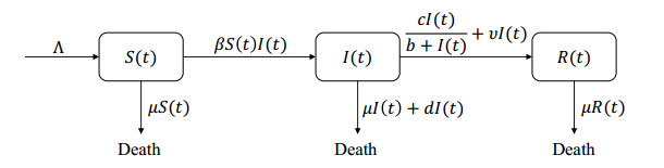
The classic SIR model is often used to evaluate the effectiveness of controlling infectious diseases. Moreover, when adopting strategies such as isolation and vaccination based on changes in the size of susceptible populations and other states, it is necessary to develop a non-smooth SIR infectious disease model. To do this, we first add a non-linear term to the classical SIR model to describe the impact of limited medical resources or treatment capacity on infectious disease transmission, and then involve the state-dependent impulsive feedback control, which is determined by the convex combinations of the size of the susceptible population and its growth rates, into the model. Further, the analytical methods have been developed to address the existence of non-trivial periodic solutions, the existence and stability of a disease-free periodic solution (DFPS) and its bifurcation. Based on the properties of the established Poincaré map, we conclude that DFPS exists, which is stable under certain conditions. In particular, we show that the non-trivial order-1 periodic solutions may exist and a non-trivial order-$ k $ ($ k\geq 1 $) periodic solution in some special cases may not exist. Moreover, the transcritical bifurcations around the DFPS with respect to the parameters $ p $ and $ AT $ have been investigated by employing the bifurcation theorems of discrete maps.
Citation: Chenxi Huang, Qianqian Zhang, Sanyi Tang. Non-smooth dynamics of a SIR model with nonlinear state-dependent impulsive control[J]. Mathematical Biosciences and Engineering, 2023, 20(10): 18861-18887. doi: 10.3934/mbe.2023835
The classic SIR model is often used to evaluate the effectiveness of controlling infectious diseases. Moreover, when adopting strategies such as isolation and vaccination based on changes in the size of susceptible populations and other states, it is necessary to develop a non-smooth SIR infectious disease model. To do this, we first add a non-linear term to the classical SIR model to describe the impact of limited medical resources or treatment capacity on infectious disease transmission, and then involve the state-dependent impulsive feedback control, which is determined by the convex combinations of the size of the susceptible population and its growth rates, into the model. Further, the analytical methods have been developed to address the existence of non-trivial periodic solutions, the existence and stability of a disease-free periodic solution (DFPS) and its bifurcation. Based on the properties of the established Poincaré map, we conclude that DFPS exists, which is stable under certain conditions. In particular, we show that the non-trivial order-1 periodic solutions may exist and a non-trivial order-$ k $ ($ k\geq 1 $) periodic solution in some special cases may not exist. Moreover, the transcritical bifurcations around the DFPS with respect to the parameters $ p $ and $ AT $ have been investigated by employing the bifurcation theorems of discrete maps.

| [1] |
B. Fatima, M. Yavuz, M. ur Rahman, and F.S. Al-Duais. Modeling the epidemic trend of middle eastern respiratory syndrome coronavirus with optimal control. Math. Biosci. Eng., 20 (2023), 11847–11874. http://doi.org/10.3934/mbe.2023527 doi: 10.3934/mbe.2023527

|
| [2] |
F. Evirgen, E. Uçar, S. Uçar, N. $\mathrm{\ddot{O}}$zdemir, Modelling influenza a disease dynamics under Caputo–Fabrizio fractional derivative with distinct contact rates, Math. Mod. Numer. Simul. Appl., 3 (2023), 58–73. https://doi.org/10.53391/mmnsa.1274004 doi: 10.53391/mmnsa.1274004
|
| [3] |
H. Joshi, M. Yavuz, S. Townley, B. K. Jha, Stability analysis of a non-singular fractional-order covid-19 model with nonlinear incidence and treatment rate, Phys. Scr., 98 (2023), 045216. https://doi.org/10.1088/1402-4896/acbe7a doi: 10.1088/1402-4896/acbe7a
|
| [4] |
A. G. C. Pérez, D. A. Oluyori, A model for COVID-19 and bacterial pneumonia coinfection with community- and hospital-acquired infections, Math. Mod. Numer. Simul. Appl., 2 (2022), 197–210. https://doi.org/10.53391/mmnsa.2022.016 doi: 10.53391/mmnsa.2022.016
|
| [5] |
A. O. Atede, A. Omame, S. C. Inyama, A fractional order vaccination model for COVID-19 incorporating environmental transmission: a case study using Nigerian data, Bull. Math. Biol., 1 (2023), 78–110. https://doi.org/10.59292/bulletinbiomath.2023005 doi: 10.59292/bulletinbiomath.2023005
|
| [6] |
J. A. Cui, X. X. Mu, H. Wan, Saturation recovery leads to multiple endemic equilibria and backward bifurcation, J. Theoret. Biol., 254 (2008), 275–283. https://doi.org/10.1016/j.jtbi.2008.05.015 doi: 10.1016/j.jtbi.2008.05.015
|
| [7] |
H. Wan, J. A. Cui, Rich dynamics of an epidemic model with saturation recovery, J. Appl. Math., 2013 (2013), 314958. https://doi.org/10.1155/2013/314958 doi: 10.1155/2013/314958
|
| [8] |
N. C. Grassly, C. Fraser, Mathematical models of infectious disease transmission, Nat. Rev. Microbiol., 6 (2008), 477–487. https://doi.org/10.1038/nrmicro1845 doi: 10.1038/nrmicro1845
|
| [9] |
G. R. Jiang, Q. G. Yang, Periodic solutions and bifurcation in an SIS epidemic model with birth pulses, Math. Comput. Model., 50 (2009), 498–508. https://doi.org/10.1016/j.mcm.2009.04.021 doi: 10.1016/j.mcm.2009.04.021
|
| [10] |
J. Yang, S. Y. Tang, Holling type Ⅱ predator-prey model with nonlinear pulse as state-dependent feedback control, J. Comput. Appl. Math., 291 (2016), 225–241. https://doi.org/10.1016/j.cam.2015.01.017 doi: 10.1016/j.cam.2015.01.017
|
| [11] |
Q. Q. Zhang, S. Y. Tang, X. F. Zou, Rich dynamics of a predator-prey system with state-dependent impulsive controls switching between two means, J. Differ. Equation, 364 (2023), 336–377. https://doi.org/10.1016/j.jde.2023.03.030 doi: 10.1016/j.jde.2023.03.030
|
| [12] |
Q. Q. Zhang, B. Tang, S. Y. Tang, Vaccination threshold size and backward bifurcation of SIR model with state-dependent pulse control, J. Theoret. Biol., 455 (2018), 75–85. https://doi.org/10.1016/j.jtbi.2018.07.010 doi: 10.1016/j.jtbi.2018.07.010
|
| [13] |
T. Y. Cheng, S. Y. Tang, R. A. Cheke, Threshold dynamics and bifurcation of a state-dependent feedback nonlinear control Susceptible-Infected-Recovered model, J. Comput. Dyn., 14 (2019), 1–14. https://doi.org/10.1115/1.4043001 doi: 10.1115/1.4043001
|
| [14] |
S. Y. Tang, Y. N. Xiao, D. Clancy, New modelling approach concerning integrated disease control and cost-effectivity, Nonlinear Anal., 63 (2005), 439–471. https://doi.org/10.1016/j.na.2005.05.029 doi: 10.1016/j.na.2005.05.029
|
| [15] |
S. Y. Tang, Y. N. Xiao, L. S. Chen, R. A. Cheke, Integrated pest management models and their dynamical behaviour, Bull. Math. Biol., 67 (2005), 115–135. https://doi.org/10.1016/j.bulm.2004.06.005 doi: 10.1016/j.bulm.2004.06.005
|
| [16] |
L. F. Nie, Z. D. Teng, B. Z. Guo, A state dependent pulse control strategy for a SIRS epidemic system, Bull. Math. Biol., 75 (2013), 1697–1715. https://doi.org/10.1007/s11538-013-9865-y doi: 10.1007/s11538-013-9865-y
|
| [17] |
S. Y. Tang, B. Tang, A. L. Wang, Y. N. Xiao, Holling Ⅱ predator-prey impulsive semi-dynamic model with complex poincaré map, Nonlinear Dynam., 81 (2015), 1575–1596. https://doi.org/10.1007/s11071-015-2092-3 doi: 10.1007/s11071-015-2092-3
|
| [18] |
S. Y. Tang, W. H. Pang, On the continuity of the function describing the times of meeting impulsive set and its application, Math. Biosci. Eng., 14 (2017), 1399–1406. http://doi.org/10.3934/mbe.2017072 doi: 10.3934/mbe.2017072
|
| [19] |
S. Y. Tang, C. T. Li, B. Tang, X. Wang, Global dynamics of a nonlinear state-dependent feedback control ecological model with a multiple-hump discrete map, Commun. Nonlinear Sci. Numer. Simul., 79 (2019), 104900. https://doi.org/10.1016/j.cnsns.2019.104900 doi: 10.1016/j.cnsns.2019.104900
|
| [20] |
Q. Q. Zhang, B. Tang, T. Y. Cheng, S.Y. Tang, Bifurcation analysis of a generalized impulsive kolmogorov model with applications to pest and disease control, SIAM J. Appl. Math., 80 (2020), 1796–1819. https://doi.org/10.1137/19M1279320 doi: 10.1137/19M1279320
|
| [21] |
W. Li, T. H. Zhang, Y. F. Wang, H. D. Cheng, Dynamic analysis of a plankton-herbivore state-dependent impulsive model with action threshold depending on the density and its changing rate, Nonlinear Dynam., 107 (2022), 2951–2963. https://doi.org/10.1007/s11071-021-07022-w doi: 10.1007/s11071-021-07022-w
|
| [22] |
Q. Q. Zhang, S. Y. Tang, Bifurcation analysis of an ecological model with nonlinear state-dependent feedback control by poincaré map defined in phase set, Commun. Nonlinear Sci. Numer. Simul., 108 (2022), 106212. https://doi.org/10.1016/j.cnsns.2021.106212 doi: 10.1016/j.cnsns.2021.106212
|
| [23] |
Y. Tian, Y. Gao, K. B. Sun, A fishery predator-prey model with anti-predator behavior and complex dynamics induced by weighted fishing strategies, Math. Biosci. Eng., 20 (2023), 1558–1579. http://doi.org/10.3934/mbe.2023071 doi: 10.3934/mbe.2023071
|
| [24] |
Y. Tian, Y. Gao, K. B. Sun, Qualitative analysis of exponential power rate fishery model and complex dynamics guided by a discontinuous weighted fishing strategy, Commun. Nonlinear Sci. Numer. Simul., 118 (2023), 107011. https://doi.org/10.1016/j.cnsns.2022.107011 doi: 10.1016/j.cnsns.2022.107011
|
| [25] |
A. d'Onofrio, Stability properties of pulse vaccination strategy in SEIR epidemic model, Math. Biosci., 179 (2002), 57–72. https://doi.org/10.1016/S0025-5564(02)00095-0 doi: 10.1016/S0025-5564(02)00095-0
|
| [26] |
A. d'Onofrio, On pulse vaccination strategy in the SIR epidemic model with vertical transmission, Appl. Math. Lett., 18 (2005), 729–732. https://doi.org/10.1016/j.aml.2004.05.012 doi: 10.1016/j.aml.2004.05.012
|
| [27] |
P. Cull, Global stability of population models, Bull. Math. Biol., 43 (1981), 47–58. https://doi.org/10.1016/S0092-8240(81)80005-5 doi: 10.1016/S0092-8240(81)80005-5
|
| [28] |
N. Ferguson, D. Cummings, S. Cauchemez, C. Fraser, S. Riley, A. Meeyai, et al., Strategies for containing an emerging influenza pandemic in Southeast Asia, Nature, 437 (2005), 209–214. https://doi.org/10.1038/nature04017 doi: 10.1038/nature04017
|
| [29] |
B. Shulgin, L. Stone, Z. Agur, Pulse vaccination strategy in the SIR epidemic model, Bull. Math. Biol., 60 (1998), 1123–1148. https://doi.org/10.1006/S0092-8240(98)90005-2 doi: 10.1006/S0092-8240(98)90005-2
|
| [30] |
Z. Agur, L. Cojocaru, G. Mazor, R. M. Anderson, Y. L. Danon, Pulse mass measles vaccination across age cohorts, Proc. Pakistan Acad. Sci., 90 (1993), 11698–11702. https://doi.org/10.1073/pnas.90.24.11698 doi: 10.1073/pnas.90.24.11698
|
| [31] |
F. Albrecht, H. Gatzke, A. Haddad, N. Wax, The dynamics of two interacting populations, J. Math. Anal. Appl., 46 (1974), 658–670. https://doi.org/10.1016/0016-0032(74)90039-8 doi: 10.1016/0016-0032(74)90039-8
|
| [32] |
M. E. Fisher, B. S. Goh, T. L. Vincent, Some stability conditions for discrete-time single species models, Bull. Math. Biol., 41 (1979), 861–875. https://doi.org/10.1007/BF02462383 doi: 10.1007/BF02462383
|
| [33] | S. K. Kaul, Stability and asymptotic stability in impulsive semidynamical systems, J. Appl. Math. Stoch. Anal., 7 (1994), 509–523. |
| [34] | S. K. Kaul, On impulsive semidynamical systems Ⅲ: Lyapunov stability, in Recent Trends in Differential Equations, World Scientific, (1992), 335–345. |
| [35] | D. D. Bainov, P. S. Simeonov, Impulsive differential equations: periodic solutions and applications, CRC Press, New York, 1993. |
| [36] | A. Lakmeche, Bifurcation of non trivial periodic solutions of impulsive differential equations arising chemotherapeutic treatment, Dynam. Contin. Discrete Impuls., 7 (2000), 265–287. |
| [37] |
D. Singer, Stable orbits and bifurcation of maps of the interval, SIAM J. Appl. Math., 35 (1978), 260–267. https://doi.org/10.1137/0135020 doi: 10.1137/0135020
|
| [38] | J. E. Marsden, M. McCracken, The hopf bifurcation and its applications, Springer-Verlag, New York, 2012. |
| [39] | J. M. Grandmont, Periodic and aperiodic behaviour in discrete One-Dimensional dynamical systems, Princeton University Press, Princeton, 1992. |
| [40] | S. Kaul, On impulsive semidynamical systems, J. Math. Anal. Appl., 150 (1990), 120–128. |
| [41] |
E. M. Bonotto, M. Federson, Limit sets and the Poincaré-Bendixson Theorem in impulsive semidynamical systems, J. Differ. Equation, 244 (2008), 2334–2349. https://doi.org/10.1016/j.jde.2008.02.007 doi: 10.1016/j.jde.2008.02.007
|
| [42] |
P. S. Simeonov, D. D. Bainov, Orbital stability of the periodic solutions of autonomous systems with impulse effect, Int. J. Syst. Sci., 19 (1988), 2561–2585. https://doi.org/10.2977/prims/1195173347 doi: 10.2977/prims/1195173347
|
| [43] |
J. M. Grandmont, Nonlinear difference equations, bifurcations and chaos: An introduction, Res. Econ., 62 (2008), 122–177. https://doi.org/10.1016/j.rie.2008.06.003 doi: 10.1016/j.rie.2008.06.003
|
| [44] |
H. Zhou, S. Y. Tang, Complex dynamics and sliding bifurcations of the Filippov Lorenz–Chen system, Int. J. Bifur. Chaos, 32 (2022), 2250182. https://doi.org/10.1142/S0218127422501826 doi: 10.1142/S0218127422501826
|
| [45] |
H. Zhou, S. Y. Tang, Bifurcation dynamics on the sliding vector field of a Filippov ecological system, Appl. Math. Comput., 424 (2022), 127052. https://doi.org/10.1016/j.amc.2022.127052 doi: 10.1016/j.amc.2022.127052
|


Figures(5)

Chenxi Huang, Qianqian Zhang, Sanyi Tang. Non-smooth dynamics of a SIR model with nonlinear state-dependent impulsive control[J]. Mathematical Biosciences and Engineering, 2023, 20(10): 18861-18887. doi: 10.3934/mbe.2023835


 DownLoad: