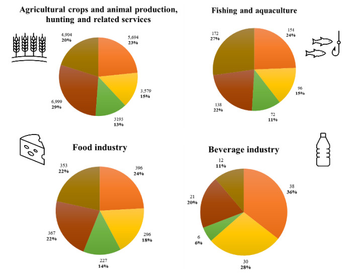
It is undeniable that the agri-food system is one of the greatest waste-producing sectors, with the inevitable generation of a certain quantity of scraps due to processing at an industrial level. Circular economy may offer a valid solution to overcome this problem, but the application of the model requires the availability of reliable data about quality and quantity of waste, which are currently missing. For this purpose, the objective of this paper is to address the issue of waste generation in the agri-food industry using a survey questionnaire. In-depth interviews were conducted with the owners or the technicians of selected case studies from the Marche region agri-food sector. Then, mass balance was applied based on primary data collected during the interviews. Moreover, to explore the potentiality of the circular model for the development of a regional agri-food sector, barriers, opportunities and services were also investigated. Results identified the vegetable and olive oil transformation as the most impacting in terms of quantities of waste produced. Food business operators currently find it difficult to give a proper definition of circular economy and envision the implementation of the model soon. However, they are also very enthusiastic and positive in finding alternative solutions to recover the waste. A great support could be provided by establishing a regional database for waste qualification and quantification. This work could be useful for policy makers, helping to understand the hurdles that agribusiness entrepreneurs shall face in this economic transition.
Citation: Giulia Chiaraluce, Deborah Bentivoglio, Adele Finco. The circular economy model in the agri-food sector: A new strategy for the regional development[J]. AIMS Agriculture and Food, 2023, 8(3): 851-872. doi: 10.3934/agrfood.2023045
It is undeniable that the agri-food system is one of the greatest waste-producing sectors, with the inevitable generation of a certain quantity of scraps due to processing at an industrial level. Circular economy may offer a valid solution to overcome this problem, but the application of the model requires the availability of reliable data about quality and quantity of waste, which are currently missing. For this purpose, the objective of this paper is to address the issue of waste generation in the agri-food industry using a survey questionnaire. In-depth interviews were conducted with the owners or the technicians of selected case studies from the Marche region agri-food sector. Then, mass balance was applied based on primary data collected during the interviews. Moreover, to explore the potentiality of the circular model for the development of a regional agri-food sector, barriers, opportunities and services were also investigated. Results identified the vegetable and olive oil transformation as the most impacting in terms of quantities of waste produced. Food business operators currently find it difficult to give a proper definition of circular economy and envision the implementation of the model soon. However, they are also very enthusiastic and positive in finding alternative solutions to recover the waste. A great support could be provided by establishing a regional database for waste qualification and quantification. This work could be useful for policy makers, helping to understand the hurdles that agribusiness entrepreneurs shall face in this economic transition.

| [1] |
Girotto, F, Alibardi, L, Cossu, R (2015) Food waste generation and industrial uses: A review. Waste Manage 45: 32–41. https://doi.org/10.1016/j.wasman.2015.06.008 doi: 10.1016/j.wasman.2015.06.008

|
| [2] |
Thyberg KL, Tonjes DJ (2016) Drivers of food waste and their implications for sustainable policy development. Resour Conserv Recycl 106: 110–123. https://doi.org/10.1016/j.resconrec.2015.11.016 doi: 10.1016/j.resconrec.2015.11.016
|
| [3] |
Giordano C, Alboni F, Falasconi L (2019) Quantities, determinants, and awareness of households' food waste in Italy: A comparison between diary and questionnaires quantities. Sustainability 11: 3381. https://doi.org/10.3390/su11123381 doi: 10.3390/su11123381
|
| [4] |
Charatsari C, Lioutas ED, De Rosa M, et al. (2022) Technological innovation and Agrifood systems resilience: The potential and perils of three different strategies. Front Sustain Food Syst 6: 872706. https://doi.org/10.3389/fsufs.2022.872706 doi: 10.3389/fsufs.2022.872706
|
| [5] |
Agnusdei L, Krstić M, Palmi P, et al. (2023) Digitalization as driver to achieve circularity in the agroindustry: A SWOT-ANP-ADAM approach. Sci Total Environ 882: 163441. https://doi.org/10.1016/j.scitotenv.2023.163441 doi: 10.1016/j.scitotenv.2023.163441
|
| [6] | Faccilongo N, Pellegrini G, La Sala P (2017) Economia circolare e scarti nelle filiere agroalimentari: Prima indagine esplorativa sullo stato dell'arte. L'industria 38: 221–240. https://www.rivisteweb.it/doi/10.1430/87786 |
| [7] | Hall KD, Guo J, Dore M, et al. (2009) The progressive increase of food waste in America and its environmental impact. PloS one 4: e7940. https://doi.org/10.1371/journal.pone.0007940 |
| [8] |
Scherhaufer S, Moates G, Hartikainen H, et al. (2018) Environmental impacts of food waste in Europe. Waste Manage 77: 98–113. https://doi.org/10.1016/j.wasman.2018.04.038 doi: 10.1016/j.wasman.2018.04.038
|
| [9] |
Tonini D, Albizzati PF, Astrup TF (2018) Environmental impacts of food waste: Learnings and challenges from a case study on UK. Waste Manage 76: 744–766. https://doi.org/10.1016/j.wasman.2018.03.032 doi: 10.1016/j.wasman.2018.03.032
|
| [10] | Venkat K (2012) The climate change and economic impacts of food waste in the United States. Int J Food Syst Dyn 2: 431–446. |
| [11] |
Stancu V, Haugaard P, Lähteenmäki L (2016) Determinants of consumer food waste behaviour: Two routes to food waste. Appetite 96: 7–17. https://doi.org/10.1016/j.appet.2015.08.025 doi: 10.1016/j.appet.2015.08.025
|
| [12] |
Rosenberg M (2021) Thoughts about food security, food loss and waste and what has to be done. AIMS Agric Food 6: 797–798. https://doi.org/10.3934/agrfood.2021048 doi: 10.3934/agrfood.2021048
|
| [13] |
Hamilton HA, Peverill MS, Müller DB, et al. (2015) Assessment of food waste prevention and recycling strategies using a multilayer systems approach. Envir Sci Tech 49: 13937–13945. https://doi.org/10.1021/acs.est.5b03781 doi: 10.1021/acs.est.5b03781
|
| [14] |
Cristóbal J, Castellani V, Manfredi S, et al. (2018) Prioritizing and optimizing sustainable measures for food waste prevention and management. Waste Manage 72: 3–16. https://doi.org/10.1016/j.wasman.2017.11.007 doi: 10.1016/j.wasman.2017.11.007
|
| [15] |
Tavill G (2020) Industry challenges and approaches to food waste. Physiol Behav 223: 112993. https://doi.org/10.1016/j.physbeh.2020.112993 doi: 10.1016/j.physbeh.2020.112993
|
| [16] | FAO (2019) The State of Food and Agriculture 2019. Moving forward on food loss and waste reduction. Food and Agriculture Organization of the United Nations, Rome. Licence: CC BY-NC-SA 3.0 IGO. Available from: https://www.fao.org/3/ca6030en/ca6030en.pdf. |
| [17] |
Papargyropoulou E, Lozano R, Steinberger JK, et al. (2014) The food waste hierarchy as a framework for the management of food surplus and food waste. J Cleaner Prod 76: 106–115. https://doi.org/10.1016/j.jclepro.2014.04.020 doi: 10.1016/j.jclepro.2014.04.020
|
| [18] |
Ghisellini P, Cialani C, Ulgiati S (2016) A review on circular economy: the expected transition to a balanced interplay of environmental and economic systems. J Cleaner Prod 114: 11–32. https://doi.org/10.1016/j.jclepro.2015.09.007 doi: 10.1016/j.jclepro.2015.09.007
|
| [19] |
Teigiserova DA, Hamelin L, Thomsen M (2020) Towards transparent valorization of food surplus, waste and loss: Clarifying definitions, food waste hierarchy, and role in the circular economy. Sci Total Environ 706: 136033. https://doi.org/10.1016/j.scitotenv.2019.136033 doi: 10.1016/j.scitotenv.2019.136033
|
| [20] |
Kusumowardani N, Tjahjono B, Lazell J, et al. (2022) A circular capability framework to address food waste and losses in the agri-food supply chain: The antecedents, principles and outcomes of circular economy J Bus Res 142: 17–31. https://doi.org/10.1016/j.jbusres.2021.12.020 doi: 10.1016/j.jbusres.2021.12.020
|
| [21] |
Lucia C, Laudicina VA, Badalucco L, et al. (2022) Challenges and opportunities for citrus wastewater management and valorisation: A review. J Environ Manage 321: 115924. https://doi.org/10.1016/j.jenvman.2022.115924 doi: 10.1016/j.jenvman.2022.115924
|
| [22] |
Andersen MS (2007) An introductory note on the environmental economics of the circular economy. Sustain Sci 2: 133–140. https://doi.org/10.1007/s11625-006-0013-6 doi: 10.1007/s11625-006-0013-6
|
| [23] | Koumparou D (2017) Circular economy and social sustainability. In: Proceedings of the Solid Waste Management & its Contribution to Circular Economy, Athens, Greece, 14–15. |
| [24] | Velenturf AP, Purnell P (2021) Principles for a sustainable circular economy. Sustain Prod Consum 27: 1437–1457. https://doi.org/10.1016/j.spc.2021.02.018 |
| [25] |
Camilleri MA (2020) European environment policy for the circular economy: Implications for business and industry stakeholders. Sustain Dev 28: 1804–1812. https://doi.org/10.1002/sd.2113 doi: 10.1002/sd.2113
|
| [26] |
Eckert E, Kovalevska O (2021) Sustainability in the European Union: Analyzing the discourse of the European green deal. J Risk Financ Manag 14: 80. https://doi.org/10.3390/jrfm14020080 doi: 10.3390/jrfm14020080
|
| [27] |
Kuci A, Fogarassy C (2021) European green deal policy for the circular economy opportunities and challenges. Hung Agric Eng 39: 65–73. https://doi.org/10.17676/HAE.2021.39.65 doi: 10.17676/HAE.2021.39.65
|
| [28] |
Riccaboni A, Neri E, Trovarelli F, et al. (2021) Sustainability-oriented research and innovation in 'farm to fork' value chains. Curr Opin Food Sci 42: 102–112. https://doi.org/10.1016/j.cofs.2021.04.006 doi: 10.1016/j.cofs.2021.04.006
|
| [29] |
Fiore M, Sauvée L, Wiśniewska-Paluszak J (2022) Opportunities and challenges of EU farm-to-fork strategy. Int Food Agribus Man Rev 25: 703–707. https://doi.org/10.22434/IFAMR2022.x001 doi: 10.22434/IFAMR2022.x001
|
| [30] |
Esposito B, Sessa MR, Sica D, et al. (2020) Towards circular economy in the agri-food sector. A systematic literature review. Sustainability 12: 7401. https://doi.org/10.3390/su12187401 doi: 10.3390/su12187401
|
| [31] | European Parliament (2008) Directive 2008/98/EC of the European Parliament and of the Council of 19 November 2008 on waste and repealing certain Directives. European Parliament. Available from: https://eur-lex.europa.eu/legal-content/EN/TXT/PDF/?uri = CELEX: 02008L0098-20180705. |
| [32] |
Chiaraluce G (2021) Circular economy in the agri-food sector: A policy overview. Ital Rev Agric Econ 76: 53–60. https://doi.org/10.36253/rea-13375 doi: 10.36253/rea-13375
|
| [33] |
Parfitt J, Barthel M, Macnaughton S (2010) Food waste within food supply chains: Quantification and potential for change to 2050. Phil Trans R Soc B 365: 3065–3081. https://doi.org/10.1098/rstb.2010.0126 doi: 10.1098/rstb.2010.0126
|
| [34] |
Alamar MDC, Falagán N, Aktas E, et al. (2018) Minimising food waste: A call for multidisciplinary research. J Sci Food Agr 98: 8–11. https://doi.org/10.1002/jsfa.8708 doi: 10.1002/jsfa.8708
|
| [35] |
Ioannou A, Georgali PZ, Fokaides PA (2022) Quantification of food waste in an insular island state for all stages of the food supply chain. Resour Conserv Recycl 185: 106486. https://doi.org/10.1016/j.resconrec.2022.106486 doi: 10.1016/j.resconrec.2022.106486
|
| [36] |
Ju M, Osako M, Harashina S (2017) Food loss rate in food supply chain using material flow analysis. Waste Manage 61: 443–454. https://doi.org/10.1016/j.wasman.2017.01.021 doi: 10.1016/j.wasman.2017.01.021
|
| [37] |
Caldeira C, De Laurentiis V, Corrado S, et al. (2019) Quantification of food waste per product group along the food supply chain in the European Union: A mass flow analysis. Resour Conserv Recycl 149: 479–488. https://doi.org/10.1016/j.resconrec.2019.06.011 doi: 10.1016/j.resconrec.2019.06.011
|
| [38] |
Amicarelli V, Bux C, Lagioia G (2020) How to measure food loss and waste? A material flow analysis application. Brit Food J 123: 67–85. https://doi.org/10.1108/BFJ-03-2020-0241 doi: 10.1108/BFJ-03-2020-0241
|
| [39] | CREA (2022) L'agricoltura italiana conta. CREA. Available from: https://www.crea.gov.it/web/politiche-e-bioeconomia/-/agricoltura-italiana-conta. |
| [40] |
Mirabella N, Castellani V, Sala S (2014) Current options for the valorization of food manufacturing waste: A review. J Cleaner Prod 65: 28–41. https://doi.org/10.1016/j.jclepro.2013.10.051 doi: 10.1016/j.jclepro.2013.10.051
|
| [41] |
Ncube A, Fiorentino G, Panfilo C, et al. (2022) Circular economy paths in the olive oil industry: A Life Cycle Assessment look into environmental performance and benefits. Int J Life Cycle Assess 2022: 1–21. https://doi.org/10.1007/s11367-022-02031-2 doi: 10.1007/s11367-022-02031-2
|
| [42] |
Ktori R, Kamaterou P, Zabaniotou A (2018) Spent coffee grounds valorization through pyrolysis for energy and materials production in the concept of circular economy. Mater Today-Proc 5: 27582–27588. https://doi.org/10.1016/j.matpr.2018.09.078 doi: 10.1016/j.matpr.2018.09.078
|
| [43] |
van Keulen M, Kirchherr J (2021) The implementation of the circular economy: Barriers and enablers in the coffee value chain J Cleaner Prod 281: 125033. https://doi.org/10.1016/j.jclepro.2020.125033 doi: 10.1016/j.jclepro.2020.125033
|
| [44] |
La Scalia G, Saeli M, Miglietta PP, et al. (2021) Coffee biowaste valorization within circular economy: An evaluation method of spent coffee grounds potentials for mortar production. Int J Life Cycle Assess 26: 1805–1815. https://doi.org/10.1007/s11367-021-01968-0 doi: 10.1007/s11367-021-01968-0
|
| [45] |
Mayson S, Williams ID (2021) Applying a circular economy approach to valorize spent coffee grounds. Resour Conserv Recycl 172: 105659. https://doi.org/10.1016/j.resconrec.2021.105659 doi: 10.1016/j.resconrec.2021.105659
|
| [46] |
Shrikhande AJ (2000) Wine by-products with health benefits. Food Res Int 33: 469–474. https://doi.org/10.1016/S0963-9969(00)00071-5 doi: 10.1016/S0963-9969(00)00071-5
|
| [47] |
Teixeira A, Baenas N, Dominguez-Perles R, et al. (2014) Natural bioactive compounds from winery by-products as health promoters: A review. Int J Mol Sci 15: 15638–15678. https://doi.org/10.3390/ijms150915638 doi: 10.3390/ijms150915638
|
| [48] |
Soto ML, Falqué E, Domínguez H (2015) Relevance of natural phenolics from grape and derivative products in the formulation of cosmetics. Cosmetics 2: 259–276. https://doi.org/10.3390/cosmetics2030259 doi: 10.3390/cosmetics2030259
|
| [49] |
Kalli E, Lappa I, Bouchagier P, et al. (2018) Novel application and industrial exploitation of winery by-products. Bioresour Bioprocess 5: 1–21. https://doi.org/10.1186/s40643-018-0232-6 doi: 10.1186/s40643-018-0232-6
|
| [50] | Yin RK (2018) Case study research and applications—Design and Methods, 6 Eds., Thousand Oaks, CA: SAGE Publications Inc. |
| [51] |
Noor KBM (2008) Case study: A strategic research methodology. Am J Appl Sci 5: 1602–1604. https://doi.org/10.3844/ajassp.2008.1602.1604 doi: 10.3844/ajassp.2008.1602.1604
|
| [52] | European Commission (2019) Commission Delegated Decision (EU) 2019/1597 of 3 May 2019 supplementing Directive 2008/98/EC of the European Parliament and of the Council as regards a common methodology and minimum quality requirements for the uniform measurement of levels of food waste. European Commission. Available from: https://eur-lex.europa.eu/legal-content/EN/TXT/PDF/?uri = CELEX: 32019D1597. |
| [53] |
Tisserant A, Pauliuk S, Merciai S, et al. (2017) Solid waste and the circular economy: A global analysis of waste treatment and waste footprints. J Ind Ecol 21: 628–640. https://doi.org/10.1111/jiec.12562 doi: 10.1111/jiec.12562
|
| [54] |
Morea D, Fortunati S, Cappa F, et al. (2023) Corporate social responsibility as a catalyst of circular economy? A case study perspective in Agri-food. J Knowl Manag 27: 1787–1809. https://doi.org/10.1108/JKM-06-2022-0451 doi: 10.1108/JKM-06-2022-0451
|
| [55] | Berardi PC, Betiol LS, Dias JM (2021) From the vine to the bottle: How circular is the wine sector? A glance over waste. In: Mor RS, Panghal A, Kumar V (Eds.), Challenges and Opportunities of Circular Economy in Agri-Food Sector: Rethinking Waste, Springer, 151–175. https://doi.org/10.1007/978-981-16-3791-9_9 |
| [56] | MIPAAF (2008) Decreto n. 5396 del 27 novembre 2008 Disposizioni di attuazione dei regolamenti CE) n. 479/2008 del Consiglio e (CE) n.555/2008 della Commissione per quanto riguarda l'applicazione della misura della distillazione dei sottoprodotti della vinificazione. Ministero delle Politiche Agricole, Ambientali e Forestali. Available from: https://www.gazzettaufficiale.it/atto/serie_generale/caricaDettaglioAtto/originario?atto.dataPubblicazioneGazzetta = 2008-12-27 & atto.codiceRedazionale = 08A09953 & elenco30giorni = false. |
| [57] | Presidenza della Repubblica Italiana (1996) Legge 11 novembre 1996, n. 574. Nuove norme in materia di utilizzazione agronomica delle acque di vegetazione e di scarichi dei frantoi oleari. Available from: https://www.gazzettaufficiale.it/atto/serie_generale/caricaDettaglioAtto/originario?atto.dataPubblicazioneGazzetta = 1996-11-12 & atto.codiceRedazionale = 096G0597 & elenco30giorni = false. |
| [58] | MIPAAF (2005) Decreto 6 luglio 2005 Criteri e norme tecniche generali per la disciplina regionale dell'utilizzazione agronomica delle acque di vegetazione e degli scarichi dei frantoi oleari, di cui all'articolo 38 del decreto legislativo 11 maggio 1999, n. 152. Ministero delle Politiche Agricole, Ambientali e Forestali. Available from: https://www.gazzettaufficiale.it/eli/id/2005/07/19/05A07191/sg. |
| [59] | Heimerl F, Lohmann S, Lange S, et al. (2014) Word cloud explorer: Text analytics based on word clouds. In: 2014 47th Hawaii international conference on system sciences, IEEE, 1833–1842. https://doi.org/10.1109/HICSS.2014.231 |
| [60] | Nerantzis ET, Tataridis P (2006) Integrated enology-utilization of winery by-products into high added value products. J Sci Tech 1: 79–89. |
| [61] |
Berbel J, Posadillo A (2018) Review and analysis of alternatives for the valorisation of agro-industrial olive oil by-products. Sustainability 10: 237. https://doi.org/10.3390/su10010237 doi: 10.3390/su10010237
|
| [62] |
Principato L, Ruini L, Guidi M, et al. (2019) Adopting the circular economy approach on food loss and waste: The case of Italian pasta production. Resour Conserv Recycl 144: 82–89. https://doi.org/10.1016/j.resconrec.2019.01.025 doi: 10.1016/j.resconrec.2019.01.025
|
| [63] |
Wen L, Álvarez C, Zhang Z, et al. (2021) Optimisation and characterisation of protein extraction from coffee silverskin assisted by ultrasound or microwave techniques. Biomass Convers Bioref 11: 1575–1585. https://doi.org/10.1007/s13399-020-00712-2 doi: 10.1007/s13399-020-00712-2
|
| [64] |
Garrone P, Melacini M, Perego A, et al. (2016) Reducing food waste in food manufacturing companies. J Cleaner Prod 137: 1076–1085. https://doi.org/10.1016/j.jclepro.2016.07.145 doi: 10.1016/j.jclepro.2016.07.145
|
| [65] | FAO (2011) Global food losses and food waste—Extent, causes and prevention. Rome. Available from: https://www.fao.org/3/i2697e/i2697e.pdf. |
| [66] |
Bentivoglio D, Chiaraluce G, Finco A (2022) Economic assessment for vegetable waste valorization through the biogas-biomethane chain in Italy with a circular economy approach. Front Sustain Food Syst 6: 1035357. https://doi.org/10.3389/fsufs.2022.1035357 doi: 10.3389/fsufs.2022.1035357
|
| [67] |
Maranesi C, De Giovanni P (2020) Modern circular economy: Corporate strategy, supply chain, and industrial symbiosis. Sustainability 12: 9383. https://doi.org/10.3390/su12229383 doi: 10.3390/su12229383
|
| [68] |
Zarbà C, Chinnici G, La Via G, et al. (2021) Regulatory elements on the circular economy: Driving into the agri-food system. Sustainability 13: 8350. https://doi.org/10.3390/su13158350 doi: 10.3390/su13158350
|
| [69] |
Mhatre P, Panchal R, Singh A, et al. (2021) A systematic literature review on the circular economy initiatives in the European Union. Sustain Prod Consum 26: 187–202. https://doi.org/10.1016/j.spc.2020.09.008 doi: 10.1016/j.spc.2020.09.008
|
| [70] |
Morone P, Koutinas A, Gathergood N, et al. (2019) Food waste: Challenges and opportunities for enhancing the emerging bio-economy. J Cleaner Prod 221: 10–16. https://doi.org/10.1016/j.jclepro.2019.02.258 doi: 10.1016/j.jclepro.2019.02.258
|
| [71] |
Osorio LLDR, Flórez-López E, Grande-Tovar CD (2021) The potential of selected agri-food loss and waste to contribute to a circular economy: Applications in the food, cosmetic and pharmaceutical industries. Molecules 26: 515. https://doi.org/10.3390/molecules26020515 doi: 10.3390/molecules26020515
|
| [72] | Rizos V, Behrens A, Kafyeke T, et al. (2015) The circular economy: barriers and opportunities for SMEs. CEPS Working Documents 412. |
| [73] |
Ormazabal M, Prieto-Sandoval V, Puga-Leal R, et al. (2018) Circular economy in Spanish SMEs: Challenges and opportunities. J Cleaner Prod 185: 157–167. https://doi.org/10.1016/j.jclepro.2018.03.031 doi: 10.1016/j.jclepro.2018.03.031
|
| [74] |
Mehmood A, Ahmed S, Viza E, et al. (2021) Drivers and barriers towards circular economy in agri‐food supply chain: A review. Bus Strat Dev 4: 465–481. https://doi.org/10.1002/bsd2.171 doi: 10.1002/bsd2.171
|
| [75] |
Korhonen J, Honkasalo A, Seppälä J (2018) Circular economy: The concept and its limitations. Ecol Econ 143: 37–46. https://doi.org/10.1016/j.ecolecon.2017.06.041 doi: 10.1016/j.ecolecon.2017.06.041
|
| [76] |
Muscio A, Sisto R (2020) Are agri-food systems really switching to a circular economy model? Implications for European research and innovation policy. Sustainability 12: 5554. https://doi.org/10.3390/su12145554 doi: 10.3390/su12145554
|
| [77] |
Geissdoerfer M, Savaget P, Bocken NM, et al. (2017) The Circular Economy–A new sustainability paradigm?. J Cleaner Prod 143: 757–768. https://doi.org/10.1016/j.jclepro.2016.12.048 doi: 10.1016/j.jclepro.2016.12.048
|
| [78] |
Campos DA, Gómez-García R, Vilas-Boas AA, et al. (2020) Management of fruit industrial by-products—A case study on circular economy approach. Molecules 25: 320. https://doi.org/10.3390/molecules25020320 doi: 10.3390/molecules25020320
|
| [79] |
Chiaraluce G, Bentivoglio D, Finco A (2021) Circular economy for a sustainable agri-food supply chain: A review for current trends and future pathways. Sustainability 13: 9294. https://doi.org/10.3390/su13169294 doi: 10.3390/su13169294
|


Figures(4) / Tables(2)

Giulia Chiaraluce, Deborah Bentivoglio, Adele Finco. The circular economy model in the agri-food sector: A new strategy for the regional development[J]. AIMS Agriculture and Food, 2023, 8(3): 851-872. doi: 10.3934/agrfood.2023045


 DownLoad: