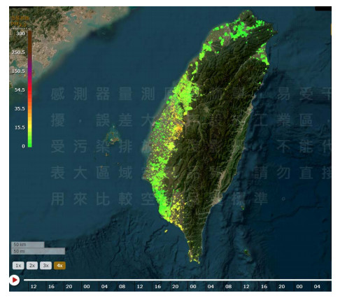
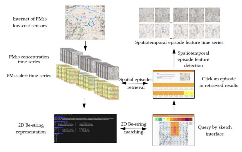
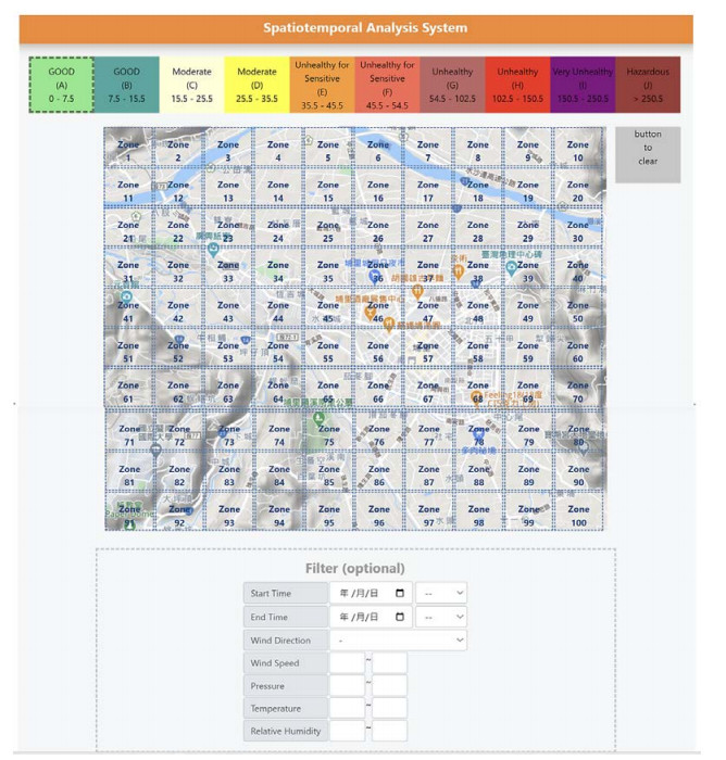
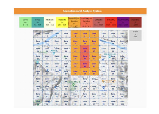
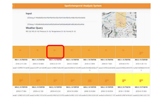
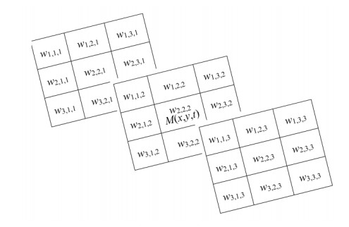
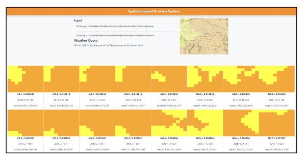
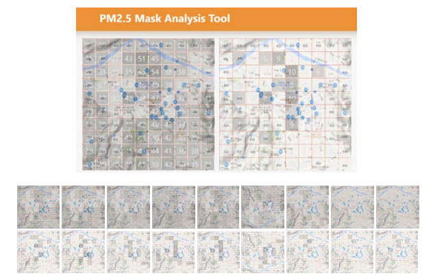
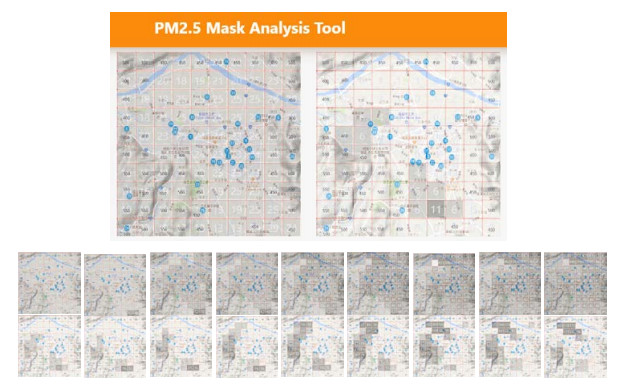
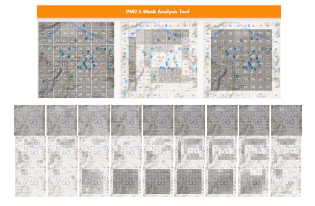
Air pollution has inevitably come along with the economic development of human society. How to balance economic growth with a sustainable environment has been a global concern. The ambient PM2.5 (particulate matter with aerodynamic diameter ≤ 2.5 μm) is particularly life-threatening because these tiny aerosols could be inhaled into the human respiration system and cause millions of premature deaths every year. The focus of most relevant research has been placed on apportionment of pollutants and the forecast of PM2.5 concentration measures. However, the spatiotemporal variations of pollution regions and their relationships to local factors are not much contemplated in the literature. These local factors include, at least, land terrain, meteorological conditions and anthropogenic activities. In this paper, we propose an interactive analysis platform for spatiotemporal retrieval and feature analysis of air pollution episodes. A domain expert can interact with the platform by specifying the episode analysis intention considering various local factors to reach the analysis goals. The analysis platform consists of two main components. The first component offers a query-by-sketch function where the domain expert can search similar pollution episodes by sketching the spatial relationship between the pollution regions and the land objects. The second component helps the domain expert choose a retrieved episode to conduct spatiotemporal feature analysis in a time span. The integrated platform automatically searches the episodes most resembling the domain expert's original sketch and detects when and where the episode emerges and diminishes. These functions are helpful for domain experts to infer insights into how local factors result in particular pollution episodes.
Citation: Peng-Yeng Yin. Spatiotemporal retrieval and feature analysis of air pollution episodes[J]. Mathematical Biosciences and Engineering, 2023, 20(9): 16824-16845. doi: 10.3934/mbe.2023750
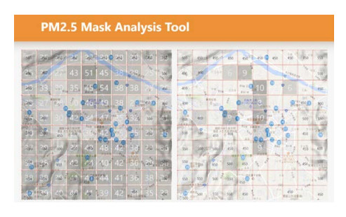
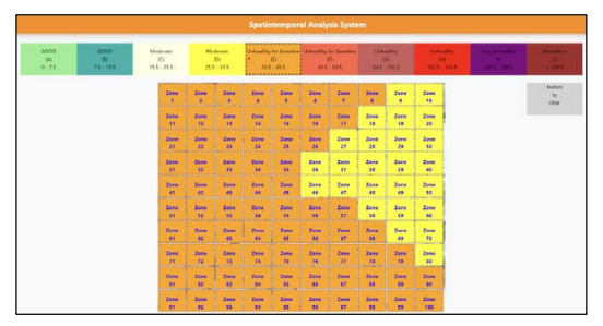
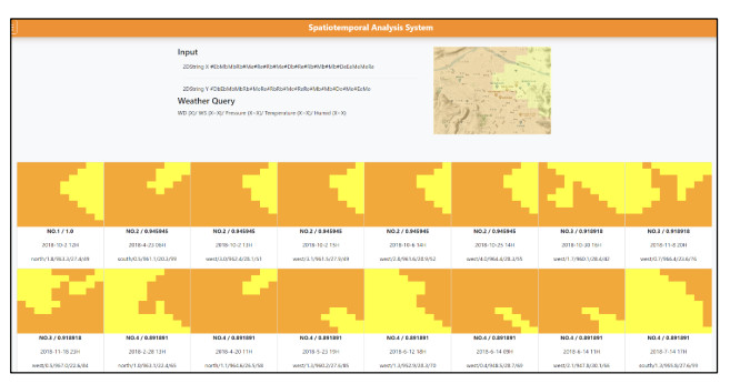
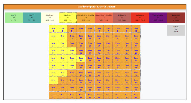
Air pollution has inevitably come along with the economic development of human society. How to balance economic growth with a sustainable environment has been a global concern. The ambient PM2.5 (particulate matter with aerodynamic diameter ≤ 2.5 μm) is particularly life-threatening because these tiny aerosols could be inhaled into the human respiration system and cause millions of premature deaths every year. The focus of most relevant research has been placed on apportionment of pollutants and the forecast of PM2.5 concentration measures. However, the spatiotemporal variations of pollution regions and their relationships to local factors are not much contemplated in the literature. These local factors include, at least, land terrain, meteorological conditions and anthropogenic activities. In this paper, we propose an interactive analysis platform for spatiotemporal retrieval and feature analysis of air pollution episodes. A domain expert can interact with the platform by specifying the episode analysis intention considering various local factors to reach the analysis goals. The analysis platform consists of two main components. The first component offers a query-by-sketch function where the domain expert can search similar pollution episodes by sketching the spatial relationship between the pollution regions and the land objects. The second component helps the domain expert choose a retrieved episode to conduct spatiotemporal feature analysis in a time span. The integrated platform automatically searches the episodes most resembling the domain expert's original sketch and detects when and where the episode emerges and diminishes. These functions are helpful for domain experts to infer insights into how local factors result in particular pollution episodes.

| [1] | United Nations. Department of Economic and Social Affairs. The 2030 Agenda for Sustainable Development. Available online: https://sdgs.un.org/goals (accessed on 30 July, 2023). |
| [2] | WHO Media Centre. Ambient (Outdoor) Air Quality and Health. 2016. Available online: http://www.who.int/mediacentre/factsheets/fs313/en/ (accessed on 30 July, 2023). |
| [3] |
N. Singh, V. Murari, M. Kumar, S. C. Barman, T. Banerjee, Fine particulates over South Asia: Review and meta-analysis of PM2.5 source apportionment through receptor model, Environ. Pollut., 223 (2017), 121–136. https://doi.org/10.1016/j.envpol.2016.12.071 doi: 10.1016/j.envpol.2016.12.071

|
| [4] |
Y. J. Han, H. W. Kim, S. H. Cho, P. R. Kim, W. J. Kim, Metallic elements in PM2.5 in different functional areas of Korea: Concentrations and source identification, Atmosph. Res., 153 (2015), 416–428. https://doi.org/10.1016/j.atmosres.2014.10.002 doi: 10.1016/j.atmosres.2014.10.002
|
| [5] |
P. Pipalatkar, V. V. Khaparde, D. G. Gajghate, M. A. Bawase, Source apportionment of PM2.5 using a CMB model for a centrally located Indian City, Aerosol Air Qual. Res., 14 (2014), 1089–1099. https://doi.org/10.4209/aaqr.2013.04.0130 doi: 10.4209/aaqr.2013.04.0130
|
| [6] |
J. Matawle, S. Pervez, S. Dewangan, S. Tiwari, D. S. Bisht, Y. F. Pervez, PM2.5 chemical source profiles of emissions resulting from industrial and domestic burning activities in India, Aerosol Air Qual. Res., 14 (2014), 2051–2066. https://doi.org/10.4209/aaqr.2014.03.0048 doi: 10.4209/aaqr.2014.03.0048
|
| [7] |
W. Chang, J. Zhan, The association of weather patterns with haze episodes: Recognition by PM2.5 oriented circulation classification applied in Xiamen, Southeastern China, Atmosph. Res., 197 (2017), 425–436. https://doi.org/10.1016/j.atmosres.2017.07.024 doi: 10.1016/j.atmosres.2017.07.024
|
| [8] |
H. L. Yu, C. H. Wang, Retrospective prediction of intra-urban spatiotemporal distribution of PM2.5 in Taipei, Atmospheric Environment, 44 (2010), 3053–3065. https://doi.org/10.1016/j.atmosenv.2010.04.034 doi: 10.1016/j.atmosenv.2010.04.034
|
| [9] |
Z. Jiang, M. D. Jolley, T. M. Fu, P. I. Palmer, Y. Ma, H. Tian, et al., Spatiotemporal and probability variations of surface PM2.5 over China between 2013 and 2019 and the associated changes in health risks: An integrative observation and model analysis, Sci. Total Environ., 723 (2020), 137896. https://doi.org/10.1016/j.scitotenv.2020.137896 doi: 10.1016/j.scitotenv.2020.137896
|
| [10] |
R. Song, L. Yang, M. Liu, C. Li, Y. Yang, Spatiotemporal Distribution of Air Pollution Characteristics in Jiangsu Province, China, Adv. Meteorol., 2019 (2019), Article ID 5907673. https://doi.org/10.1155/2019/5907673 doi: 10.1155/2019/5907673
|
| [11] |
S. C. C. Lung, W. C. V. Wang, T. Y. J. Wen, C. H. Liu, S. C. Hu, A versatile low-cost sensing device for assessing PM2.5 spatiotemporal variation and quantifying source contribution, Sci. Total Environ., 716 (2020), 137145. https://doi.org/10.1016/j.scitotenv.2020.137145 doi: 10.1016/j.scitotenv.2020.137145
|
| [12] |
D. Yang, Y. Chen, C. Miao, D. Liu, Spatiotemporal variation of PM2.5 concentrations and its relationship to urbanization in the Yangtze river delta region. China, Atmosph. Pollut. Res., 11 (2020), 491–498. https://doi.org/10.1016/j.apr.2019.11.021 doi: 10.1016/j.apr.2019.11.021
|
| [13] |
M. Habermann, M. Billger, M. Haeger-Eugensson, Land use regression as method to model air pollution. Previous results for Gothenburg/Sweden, Proced. Eng., 115 (2015), 21–28. https://doi.org/10.1016/j.proeng.2015.07.350 doi: 10.1016/j.proeng.2015.07.350
|
| [14] |
X. J. Liu, S. Y. Xia, Y. Yang, J. F. Wu, Y. N. Zhou, Y. W. Ren, Spatiotemporal dynamics and impacts of socioeconomic and natural conditions on PM2.5 in the Yangtze River Economic Belt, Environ. Pollut., 263 (2020), 114569. https://doi.org/10.1016/j.envpol.2020.114569 doi: 10.1016/j.envpol.2020.114569
|
| [15] | A. M. Dzhambov, K. Dikova, T. Georgieva, P. Mukhtarov, R. Dimitrova, Time Series Analysis of Asthma Hospital Admissions and Air Quality in Sofia - A Pilot Study, in Environmental Protection and Disaster Risks, EnviroRISKs 2022 (eds. N. Dobrinkova, O. Nikolov), Lecture Notes in Networks and Systems, 638 (2023), Springer, Cham. https://doi.org/10.1007/978-3-031-26754-3_17 |
| [16] | J. Kersey, J. Yin, Case study: Does PM2.5 contribute to the incidence of lung and bronchial cancers in the United States? in Spatiotemporal Analysis of Air Pollution and Its Application in Public Health (eds. L. Li, X. Zhou, W. Tong), Elsevier (2020), 69–89. https://doi.org/10.1016/B978-0-12-815822-7.00003-0 |
| [17] | M. Kalo, X. Zhou, L. Li, W. Tong, R. Piltner, Sensing air quality: Spatiotemporal interpolation and visualization of real-time air pollution data for the contiguous United States, in Spatiotemporal Analysis of Air Pollution and Its Application in Public Health (eds. L. Li, X. Zhou, W. Tong), Elsevier (2020), 169–196. https://doi.org/10.1016/B978-0-12-815822-7.00008-X |
| [18] |
M. Zareba, H. Dlugosz, T. Danek, E. Weglinska, Big-data-driven machine learning for enhancing spatiotemporal air pollution pattern analysis, Atmosphere, 14 (2023), 760. https://doi.org/10.3390/atmos14040760 doi: 10.3390/atmos14040760
|
| [19] |
Y. Li, T. Hong, Y. Gu, Z. Li, T. Huang, H. F. Lee, et al., Assessing the spatiotemporal characteristics, factor importance, and health impacts of air pollution in Seoul by integrating machine learning into land-use regression modeling at high spatiotemporal resolutions, Environ. Sci. Technol., 57 (2023), 1225–1236. https://doi.org/10.1021/acs.est.2c03027 doi: 10.1021/acs.est.2c03027
|
| [20] |
S. D. Chicas, J. G. Valladarez, K. Omine, Spatiotemporal distribution, trend, forecast, and influencing factors of transboundary and local air pollutants in Nagasaki Prefecture, Japan Sci. Rep., 13 (2023). https://doi.org/10.1038/s41598-023-27936-2 doi: 10.1038/s41598-023-27936-2
|
| [21] |
S. K. Chang, Q. Y. Shi, C. W. Yan, Iconic indexing by 2-D Strings, IEEE Trans. Pattern Anal. Mach. Intell., 9 (1987), 413–428. https://doi.org/10.1109/TPAMI.1987.4767923 doi: 10.1109/TPAMI.1987.4767923
|
| [22] |
Y. H. Wang, Image indexing and similarity retrieval based on spatial relationship model, Inform. Sci., 154 (2003), 39–58. https://doi.org/10.1016/S0020-0255(03)00005-7 doi: 10.1016/S0020-0255(03)00005-7
|
| [23] |
P.Y. Yin, C. C. Tsai, R. F. Day, C. Y. Tung, B. Bhanu, Ensemble learning of model hyperparameters and spatiotemporal data for calibration of low-cost PM2.5 sensors, Math. Biosci. Eng., 16 (2019), 6858–6873. https://doi.org/10.3934/mbe.2019343 doi: 10.3934/mbe.2019343
|
| [24] | R. C. Gonzalez, R. E. Woods, Digital Image Processing, 2nd Edition, Prentice Hall, New Jersey, 2002. |
| [25] | I. Giangreco, M. Springmann, I. A. Kabary, H. Schuldt, A user interface for Query-by-sketch based image retrieval with color sketches, in Advances in Information Retrieval. ECIR 2012, Lecture Notes in Computer Science, 7224 (2012), Springer, Berlin, Heidelberg. https://doi.org/10.1007/978-3-642-28997-2_67 |
| [26] |
F. Wang, S. Lin, X. Luo, B. Zhao, R. Wang, Query-by-sketch image retrieval using homogeneous painting style characterization, J. Electr. Imag., 28 (2019), 023037. https://doi.org/10.1117/1.JEI.28.2.023037 doi: 10.1117/1.JEI.28.2.023037
|
 mbe-20-09-750 supplementary.docx mbe-20-09-750 supplementary.docx |
 |

Figures(21) / Tables(1)

Peng-Yeng Yin. Spatiotemporal retrieval and feature analysis of air pollution episodes[J]. Mathematical Biosciences and Engineering, 2023, 20(9): 16824-16845. doi: 10.3934/mbe.2023750


 DownLoad: