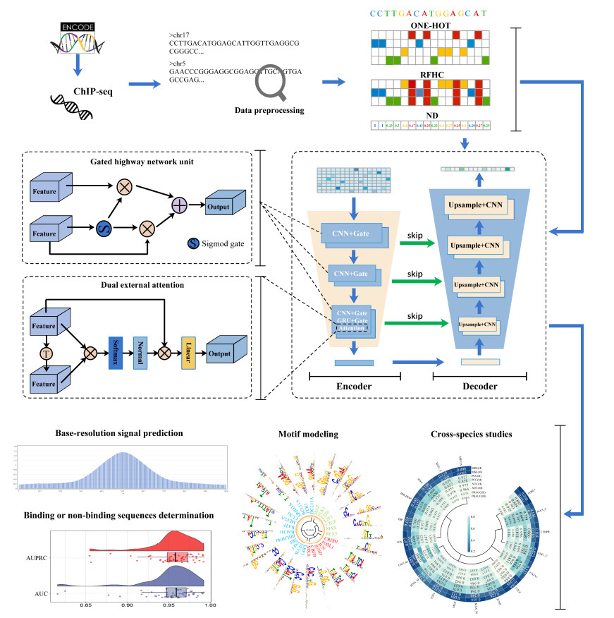
Transcription factors (TFs) are important factors that regulate gene expression. Revealing the mechanism affecting the binding specificity of TFs is the key to understanding gene regulation. Most of the previous studies focus on TF-DNA binding sites at the sequence level, and they seldom utilize the contextual features of DNA sequences. In this paper, we develop an integrated spatiotemporal context-aware neural network framework, named GNet, for predicting TF-DNA binding signal at single nucleotide resolution by achieving three tasks: single nucleotide resolution signal prediction, identification of binding regions at the sequence level, and TF-DNA binding motif prediction. GNet extracts implicit spatial contextual information with a gated highway neural mechanism, which captures large context multi-level patterns using linear shortcut connections, and the idea of it permeates the encoder and decoder parts of GNet. The improved dual external attention mechanism, which learns implicit relationships both within and among samples, and improves the performance of the model. Experimental results on 53 human TF ChIP-seq datasets and 6 chromatin accessibility ATAC-seq datasets shows that GNet outperforms the state-of-the-art methods in the three tasks, and the results of cross-species studies on 15 human and 18 mouse TF datasets of the corresponding TF families indicate that GNet also shows the best performance in cross-species prediction over the competitive methods.
Citation: Jujuan Zhuang, Kexin Feng, Xinyang Teng, Cangzhi Jia. GNet: An integrated context-aware neural framework for transcription factor binding signal at single nucleotide resolution prediction[J]. Mathematical Biosciences and Engineering, 2023, 20(9): 15809-15829. doi: 10.3934/mbe.2023704
Transcription factors (TFs) are important factors that regulate gene expression. Revealing the mechanism affecting the binding specificity of TFs is the key to understanding gene regulation. Most of the previous studies focus on TF-DNA binding sites at the sequence level, and they seldom utilize the contextual features of DNA sequences. In this paper, we develop an integrated spatiotemporal context-aware neural network framework, named GNet, for predicting TF-DNA binding signal at single nucleotide resolution by achieving three tasks: single nucleotide resolution signal prediction, identification of binding regions at the sequence level, and TF-DNA binding motif prediction. GNet extracts implicit spatial contextual information with a gated highway neural mechanism, which captures large context multi-level patterns using linear shortcut connections, and the idea of it permeates the encoder and decoder parts of GNet. The improved dual external attention mechanism, which learns implicit relationships both within and among samples, and improves the performance of the model. Experimental results on 53 human TF ChIP-seq datasets and 6 chromatin accessibility ATAC-seq datasets shows that GNet outperforms the state-of-the-art methods in the three tasks, and the results of cross-species studies on 15 human and 18 mouse TF datasets of the corresponding TF families indicate that GNet also shows the best performance in cross-species prediction over the competitive methods.

| [1] |
G. Badis, M. F. Berger, A. A. Philippakis, S. Talukder, A. R. Gehrke, S. A. Jaeger, et al., Diversity and complexity in DNA recognition by transcription factors, Science, 324 (2009), 1720–1723. https://doi.org/10.1126/science.1162327 doi: 10.1126/science.1162327

|
| [2] |
A. Jolma, J. Yan, T. Whitington, J. Toivonen, K. R. Nitta, P. Rastas, et al., DNA-binding specificities of human transcription factors, Cell, 152 (2013), 327–339. https://doi.org/10.1016/j.cell.2012.12.009 doi: 10.1016/j.cell.2012.12.009
|
| [3] |
P. J. Mitchell, R. Tjian, Transcriptional regulation in mammalian cells by sequence-specific DNA binding proteins, Science, 245 (1989), 371–378. https://doi.org/10.1126/science.2667136 doi: 10.1126/science.2667136
|
| [4] |
L. Elnitski, V. X. Jin, P. J. Farnham, S. J. Jones, Locating mammalian transcription factor binding sites: a survey of computational and experimental techniques, Genome Res., 16 (2006), 1455–1464. https://doi.org/10.1101/gr.4140006 doi: 10.1101/gr.4140006
|
| [5] |
M. F. Berger, A. A. Philippakis, A. M. Qureshi, F. S. He, P. W. Estep, M. L. Bulyk, Compact, universal DNA microarrays to comprehensively determine transcription-factor binding site specificities, Nat. Biotechnol., 24 (2006), 1429–1435. https://doi.org/10.1038/nbt1246 doi: 10.1038/nbt1246
|
| [6] |
A. Jolma, T. Kivioja, J. Toivonen, L. Cheng, G. Wei, M. Enge, et al., Multiplexed massively parallel SELEX for characterization of human transcription factor binding specificities, Genome Res., 20 (2010), 861–873. https://doi.org/10.1101/gr.100552.109 doi: 10.1101/gr.100552.109
|
| [7] |
T. S. Furey, ChIP–seq and beyond: New and improved methodologies to detect and characterize protein–DNA interactions, Nat. Rev. Genet., 13 (2012), 840–852. https://doi.org/10.1038/nrg3306 doi: 10.1038/nrg3306
|
| [8] |
J. D. Buenrostro, P. G. Giresi, L. C. Zaba, H. Y. Chang, W. J. Greenleaf, Transposition of native chromatin for fast and sensitive epigenomic profiling of open chromatin, DNA-binding proteins and nucleosome position, Nat. Methods, 10 (2013), 1213–1218. https://doi.org/10.1038/nmeth.2688 doi: 10.1038/nmeth.2688
|
| [9] |
C. Fletez-Brant, D. Lee, A. S. McCallion, M. A. Beer, kmer-SVM: a web server for identifying predictive regulatory sequence features in genomic data sets, Nucleic Acids Res., 41 (2013), W544–W556. https://doi.org/10.1093/nar/gkt519 doi: 10.1093/nar/gkt519
|
| [10] |
M. Ghandi, D. Lee, M. Mohammad-Noori, M. A. Beer, Enhanced regulatory sequence prediction using gapped k-mer features, PLoS Comput. Biol., 10 (2014), e1003711. https://doi.org/10.1371/journal.pcbi.1003711 doi: 10.1371/journal.pcbi.1003711
|
| [11] |
T. L. Bailey, N. Williams, C. Misleh, W. W. Li, MEME: Discovering and analyzing DNA and protein sequence motifs, Nucleic Acids Res., 34 (2006), W369–W373. https://doi.org/10.1093/nar/gkl198 doi: 10.1093/nar/gkl198
|
| [12] |
T. L. Bailey, STREME: Accurate and versatile sequence motif discovery, Bioinformatics, 37 (2021), 2834–2840. https://doi.org/10.1093/bioinformatics/btab203 doi: 10.1093/bioinformatics/btab203
|
| [13] |
Y. LeCun, Y. Bengio, G. Hinton, Deep learning, Nature, 521 (2015), 436–444. https://doi.org/10.1038/nature14539 doi: 10.1038/nature14539
|
| [14] |
D. Berrar, W. Dubitzky, Deep learning in bioinformatics and biomedicine, Briefings Bioinf., 22 (2021), 1513–1514. https://doi.org/10.1093/bib/bbab087 doi: 10.1093/bib/bbab087
|
| [15] |
B. Alipanahi, A. Delong, M. T. Weirauch, B. J. Frey, Predicting the sequence specificities of DNA- and RNA-binding proteins by deep learning, Nat. Biotechnol., 33 (2015), 831–838. https://doi.org/10.1038/nbt.3300 doi: 10.1038/nbt.3300
|
| [16] |
J. Zhou, O. G. Troyanskaya, Predicting effects of noncoding variants with deep learning–based sequence model, Nat. Methods, 12 (2015), 931–934. https://doi.org/10.1038/nmeth.3547 doi: 10.1038/nmeth.3547
|
| [17] |
D. Quang, X. Xie, DanQ: a hybrid convolutional and recurrent deep neural network for quantifying the function of DNA sequences, Nucleic Acids Res., 44 (2016), e107–e107. https://doi.org/10.1093/nar/gkw226 doi: 10.1093/nar/gkw226
|
| [18] |
C. Chen, J. Hou, X. Shi, H. Yang, J. A. Birchler, J. Cheng, DeepGRN: Prediction of transcription factor binding site across cell-types using attention-based deep neural networks, BMC Bioinf., 22 (2021), 38. https://doi.org/10.1186/s12859-020-03952-1 doi: 10.1186/s12859-020-03952-1
|
| [19] |
Q. X. X. Lin, D. Thieffry, S. Jha, T. Benoukraf, TFregulomeR reveals transcription factors' context-specific features and functions, Nucleic Acids Res., 48 (2020), e10–e10. https://doi.org/10.1093/nar/gkz1088 doi: 10.1093/nar/gkz1088
|
| [20] |
Ž. Avsec, M. Weilert, A. Shrikumar, S. Krueger, A. Alexandari, K. Dalal, et al., Base-resolution models of transcription-factor binding reveal soft motif syntax, Nat. Genet., 53 (2021), 354–366. https://doi.org/10.1038/s41588-021-00782-6 doi: 10.1038/s41588-021-00782-6
|
| [21] |
Q. Zhang, Y. He, S. Wang, Z. Chen, Z. Guo, Z. Cui, et al., Base-resolution prediction of transcription factor binding signals by a deep learning framework, PLoS Comput. Biol., 18 (2022), e1009941. https://doi.org/10.1371/journal.pcbi.1009941 doi: 10.1371/journal.pcbi.1009941
|
| [22] |
P. J. Werbos, Generalization of backpropagation with application to a recurrent gas market model, Neural Networks, 1 (1988), 339–356. https://doi.org/10.1016/0893-6080(88)90007-X doi: 10.1016/0893-6080(88)90007-X
|
| [23] | R. K. Srivastava, K. Greff, J. J. C. S. Schmidhuber, Training very deep networks, arXiv preprint, (2015), arXiv: 1507.06228. https://doi.org/10.48550/arXiv.1507.06228 |
| [24] | J. G. Zilly, R. K. Srivastava, J. Koutník, J. Schmidhuber, Recurrent highway networks, arXiv preprint, (2016), arXiv: 1607.03474. https://doi.org/10.48550/arXiv.1607.03474 |
| [25] | Y. N. Dauphin, A. Fan, M. Auli, D. Grangier, Language modeling with gated convolutional networks, arXiv preprint, (2016), arXiv: 1612.08083. https://doi.org/10.48550/arXiv.1612.08083 |
| [26] | D. Bahdanau, K. Cho, Y. Bengio, Neural machine translation by jointly learning to align and translate, arXiv preprint, (2014), arXiv: 1409.0473. https://doi.org/10.48550/arXiv.1409.0473 |
| [27] | K. Xu, J. L. Ba, R. Kiros, K. Cho, A. Courville, R. Salakhutdinov, et al., Show, attend and tell: Neural image caption generation with visual attention, arXiv preprint, (2015), arXiv: 1502.03044. https://doi.org/10.48550/arXiv.1502.03044 |
| [28] |
Y. Guo, C. Li, D. Zhou, J. Cao, H. Liang, Context-aware dynamic neural computational models for accurate Poly(A) signal prediction, Neural networks, 152 (2022), 287–299. https://doi.org/10.1016/j.neunet.2022.04.025 doi: 10.1016/j.neunet.2022.04.025
|
| [29] |
Y. Guo, D. Zhou, W. Li, J. Cao, R. Nie, L. Xiong, et al., Identifying polyadenylation signals with biological embedding via self-attentive gated convolutional highway networks, Appl. Soft Comput., 103 (2021), 107133. https://doi.org/10.1016/j.asoc.2021.107133 doi: 10.1016/j.asoc.2021.107133
|
| [30] | J. Lanchantin, R. Singh, Z. Lin, Y. Qi, Deep motif: Visualizing genomic sequence classifications, arXiv preprint, (2016), arXiv: 1605.01133. https://doi.org/10.48550/arXiv.1605.01133 |
| [31] | A. Vaswani, N. Shazeer, N. Parmar, J. Uszkoreit, L. Jones, A. N. Gomez, et al., Attention is all you need, arXiv preprint, (2017), arXiv: 1706.03762. https://doi.org/10.48550/arXiv.1706.03762 |
| [32] | R. Li, Z. Wu, J. Jia, Y. Bu, H. Meng, Towards discriminative representation learning for speech emotion recognition, in Proceedings of the Twenty-Eighth International Joint Conference on Artificial Intelligence, (2019), 5060–5066. https://doi.org/10.24963/ijcai.2019/703 |
| [33] |
M. H. Guo, Z. N. Liu, T. J. Mu, S. M. Hu, Beyond self-attention: External attention using two linear layers for visual tasks, IEEE Trans. Pattern Anal. Mach. Intell., 45 (2023), 5436–5447. https://doi.org/10.1109/TPAMI.2022.3211006 doi: 10.1109/TPAMI.2022.3211006
|
| [34] |
E. A. Feingold, P. J. Good, M. S. Guyer, S. Kamholz, L. Liefer, K. Wetterstrand, The ENCODE (ENCyclopedia Of DNA elements) project, Science, 306 (2004), 636–640. https://doi.org/10.1126/science.1105136 doi: 10.1126/science.1105136
|
| [35] |
M. T. Weirauch, A. Cote, R. Norel, M. Annala, Y. Zhao, T. R. Riley, et al., Evaluation of methods for modeling transcription factor sequence specificity, Nat. Biotechnol., 31 (2013), 126–134. https://doi.org/10.1038/nbt.2486 doi: 10.1038/nbt.2486
|
| [36] |
B. Manavalan, S. Basith, T. H. Shin, L. Wei, G. Lee, Meta-4mCpred: A Sequence-based meta-predictor for accurate DNA 4mC site prediction using effective feature representation, Mol. Ther. Nucleic Acids, 16 (2019), 733–744. https://doi.org/10.1016/j.omtn.2019.04.019 doi: 10.1016/j.omtn.2019.04.019
|
| [37] |
Y. Yang, Z. Hou, Y. Wang, H. Ma, P. Sun, Z. Ma, et al., HCRNet: High-throughput circRNA-binding event identification from CLIP-seq data using deep temporal convolutional network, Briefings Bioinf., 23 (2022), bbac027. https://doi.org/10.1093/bib/bbac027 doi: 10.1093/bib/bbac027
|
| [38] |
K. Liu, W. Chen, iMRM: A platform for simultaneously identifying multiple kinds of RNA modifications, Bioinformatics, 36 (2020), 3336–3342. https://doi.org/10.1093/bioinformatics/btaa155 doi: 10.1093/bioinformatics/btaa155
|
| [39] | K. He, X. Zhang, S. Ren, J. Sun, Deep residual learning for image recognition, in 2016 IEEE Conference on Computer Vision and Pattern Recognition (CVPR), IEEE, Las Vegas, USA, (2016), 770–778. https://doi.org/10.1109/CVPR.2016.90 |
| [40] | N. Srivastava, G. Hinton, A. Krizhevsky, I. Sutskever, R. Salakhutdinov, Dropout: A simple way to prevent neural networks from overfitting, J. Mach. Learn. Res., 15 (2014), 1929–1958. |
| [41] | K. Cho, B. V. Merrienboer, D. Bahdanau, Y. J. C. S. Bengio, On the properties of neural machine translation: Encoder-decoder approaches, in Proceedings of SSST-8, Eighth Workshop on Syntax, Semantics and Structure in Statistical Translation, ACL, Doha, Qatar, (2014), 103–111. https://doi.org/10.3115/v1/W14-4012 |
| [42] | D. Kingma, J. J. C. S. Ba, Adam: A method for stochastic optimization, arXiv preprint, (2014), arXiv: 1412.6980. https://doi.org/10.48550/arXiv.1412.6980 |
| [43] |
Q. Zhang, S. Wang, Z. Chen, Y. He, Q. Liu, D. S. Huang, Locating transcription factor binding sites by fully convolutional neural network, Briefings Bioinf., 22 (2021), bbaa435. https://doi.org/10.1093/bib/bbaa435 doi: 10.1093/bib/bbaa435
|
| [44] |
I. V. Kulakovskiy, I. E. Vorontsov, I. S. Yevshin, R. N. Sharipov, A. D. Fedorova, E. I. Rumynskiy, et al., HOCOMOCO: Towards a complete collection of transcription factor binding models for human and mouse via large-scale ChIP-Seq analysis, Nucleic Acids Res., 46 (2018), D252–D259. https://doi.org/10.1093/nar/gkx1106 doi: 10.1093/nar/gkx1106
|
| [45] |
S. Gupta, J. A. Stamatoyannopoulos, T. L. Bailey, W. S. Noble, Quantifying similarity between motifs, Genome Biol., 8 (2007), R24. https://doi.org/10.1186/gb-2007-8-2-r24 doi: 10.1186/gb-2007-8-2-r24
|
| [46] | T. Mikolov, K. Chen, G. Corrado, J. J. C. S. Dean, Efficient estimation of word representations in vector space, arXiv preprint, (2013), arXiv: 1301.3781. https://doi.org/10.48550/arXiv.1301.3781 |
| [47] |
L. Deng, H. Wu, X. Liu, H. Liu, DeepD2V: A novel deep learning-based framework for predicting transcription factor binding sites from combined DNA sequence, Int. J. Mol. Sci., 22 (2021), 5521. https://doi.org/10.3390/ijms22115521 doi: 10.3390/ijms22115521
|
| [48] | M. D. Zeiler, G. W. Taylor, R. Fergus, Adaptive deconvolutional networks for mid and high level feature learning, in 2011 International Conference on Computer Vision, IEEE, Barcelona, Spain, (2011), 2018–2025. https://doi.org/10.1109/ICCV.2011.6126474 |
| [49] | M. D. Zeiler, D. Krishnan, G. W. Taylor, R. Fergus, Deconvolutional networks, in 2010 IEEE Computer Society Conference on Computer Vision and Pattern Recognition, IEEE, San Francisco, USA, (2010), 2528–2535. https://doi.org/10.1109/CVPR.2010.5539957 |
| [50] |
H. Yuan, M. Kshirsagar, L. Zamparo, Y. Lu, C. S. Leslie, BindSpace decodes transcription factor binding signals by large-scale sequence embedding, Nat. Methods, 16 (2019), 858–861. https://doi.org/10.1038/s41592-019-0511-y doi: 10.1038/s41592-019-0511-y
|
 mbe-20-09-704-supplementary.pdf mbe-20-09-704-supplementary.pdf |
 |


Figures(5) / Tables(3)

Jujuan Zhuang, Kexin Feng, Xinyang Teng, Cangzhi Jia. GNet: An integrated context-aware neural framework for transcription factor binding signal at single nucleotide resolution prediction[J]. Mathematical Biosciences and Engineering, 2023, 20(9): 15809-15829. doi: 10.3934/mbe.2023704


 DownLoad: