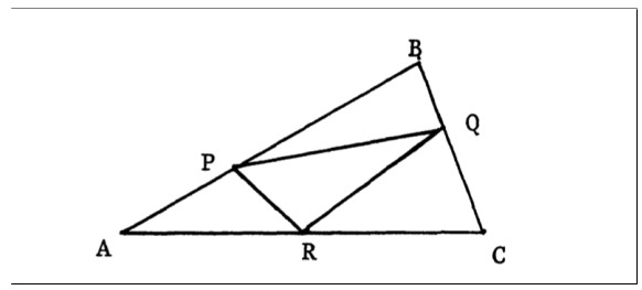
We use a quite simple, yet challenging, elementary geometry statement, the so-called "never proved" (by a mathematician) theorem, introduced by Prof. Jiawei Hong in his communication to the IEEE 1986 Symposium on Foundations of Computer Science, to exemplify and analyze the current situation of achievements, ongoing improvements and limitations of GeoGebra's automated reasoning tools, as well as other computer algebra systems, in dealing with geometric inequalities. We present a large collection of facts describing the curious (and confusing) history behind the statement and its connection to automated deduction. An easy proof of the "never proved" theorem, relying on some previous (but not trivial) human work is included. Moreover, as part of our strategy to address this challenging result with automated tools, we formulate a large list of variants of the "never proved" statement (generalizations, special cases, etc.). Addressing such variants with GeoGebra Discovery, ${\texttt{Maple}}$, ${\texttt{REDUCE/Redlog}}$ or ${\texttt{Mathematica}}$ leads us to introduce and reflect on some new approaches (e.g., partial elimination of quantifiers, consideration of symmetries, relevance of discovery vs. proving, etc.) that could be relevant to consider for future improvements of automated reasoning in geometry algorithms. As a byproduct, we obtain an original result (to our knowledge) concerning the family of triangles inscribable in a given triangle.
Citation: Zoltán Kovács, Tomás Recio, Carlos Ueno, Róbert Vajda. The "never-proved" triangle inequality: A GeoGebra & CAS approach[J]. AIMS Mathematics, 2023, 8(10): 22593-22642. doi: 10.3934/math.20231151
We use a quite simple, yet challenging, elementary geometry statement, the so-called "never proved" (by a mathematician) theorem, introduced by Prof. Jiawei Hong in his communication to the IEEE 1986 Symposium on Foundations of Computer Science, to exemplify and analyze the current situation of achievements, ongoing improvements and limitations of GeoGebra's automated reasoning tools, as well as other computer algebra systems, in dealing with geometric inequalities. We present a large collection of facts describing the curious (and confusing) history behind the statement and its connection to automated deduction. An easy proof of the "never proved" theorem, relying on some previous (but not trivial) human work is included. Moreover, as part of our strategy to address this challenging result with automated tools, we formulate a large list of variants of the "never proved" statement (generalizations, special cases, etc.). Addressing such variants with GeoGebra Discovery, ${\texttt{Maple}}$, ${\texttt{REDUCE/Redlog}}$ or ${\texttt{Mathematica}}$ leads us to introduce and reflect on some new approaches (e.g., partial elimination of quantifiers, consideration of symmetries, relevance of discovery vs. proving, etc.) that could be relevant to consider for future improvements of automated reasoning in geometry algorithms. As a byproduct, we obtain an original result (to our knowledge) concerning the family of triangles inscribable in a given triangle.

| [1] | C. Abar, Z. Kovács, T. Recio, R. Vajda, Connecting Mathematica and GeoGebra to explore inequalities on planar geometric constructions, Brazilian Wolfram Technology Conference, Sa o Paulo, November, 2019. https://www.researchgate.net/profile/Zoltan_Kovacs13/publication/337499405_Abar-Kovacs-Recio-Vajdanb/data/5ddc5439299bf10c5a33438a/Abar-Kovacs-Recio-Vajda.nb |
| [2] |
P. Boutry, G. Braun, J. Narboux, Formalization of the arithmetization of Euclidean plane geometry and applications, J. Symb. Comput., 90 (2019), 149–168. https://doi.org/10.1016/j.jsc.2018.04.007 doi: 10.1016/j.jsc.2018.04.007

|
| [3] |
F. Botana, M. Hohenwarter, P. Janičić, Z. Kovács, I. Petrović, T. Recio, et al., Automated Theorem Proving in GeoGebra: Current Achievements, J. Autom. Reasoning, 55 (2015), 39–59. https://doi.org/10.1007/s10817-015-9326-4 doi: 10.1007/s10817-015-9326-4
|
| [4] |
B. Bollobás, An extremal problem for polygons inscribed in a convex curve, Can. J. Math., 19 (1967), 523–528. https://doi.org/10.4153/CJM-1967-045-5 doi: 10.4153/CJM-1967-045-5
|
| [5] | O. Bottema, R. Žž. Djordjevič, R. R. Janič, D. S. Mitrinovič, P. M. Vasic, Geometric Inequalities, Wolters-Noordhoff Publishing, Groningen, 1969. |
| [6] | C. W. Brown, An Overview of QEPCAD B: A Tool for Real Quantifier Elimination and Formula Simplification, J. Jpn. Soc. Symbolic Algebraic Comput., 10 (2003), 13–22. |
| [7] |
C. W. Brown, Z. Kovács, T. Recio, R. Vajda, M. P. Vélez, Is computer algebra ready for conjecturing and proving geometric inequalities in the classroom?, Math. Comput. Sci., 16 (2022). https://doi.org/10.1007/s11786-022-00532-9 doi: 10.1007/s11786-022-00532-9
|
| [8] | C. W. Brown, Z. Kovács, R. Vajda, Supporting proving and discovering geometric inequalities in GeoGebra by using Tarski, In: P. Janičić, Z. Kovács, (Eds.), Proceedings of the 13th International Conference on Automated Deduction in Geometry, Electronic Proceedings in Theoretical Computer Science (EPTCS), 352 (2021), 156–166. https://doi.org/10.4204/EPTCS.352.18 |
| [9] | H. S. M. Coxeter, S. L. Greitzer, Geometry Revisited, Math. Assoc. Amer., Washington, DC. 1967. |
| [10] | J. Chen, X. Z. Yang, On a Zirakzadeh inequality related to two triangles inscribed one in the other, Publikacije Elektrotehničkog Fakulteta. Serija Matematika, 4 (1993), 25–27. |
| [11] |
G. E. Collins, H. Hong, Partial Cylindrical Algebraic Decomposition for Quantifier Elimination, J. Symb. Comput., 12 (1993), 299–328. https://doi.org/10.1016/S0747-7171(08)80152-6 doi: 10.1016/S0747-7171(08)80152-6
|
| [12] | H. T. Croft, K. J. Falconer, R. K. Guy, Unsolved Problems in Geometry, Problem Books in Mathematics, Springer-Verlag, New York, 1991. |
| [13] |
P. Davis, The rise, fall, and possible transfiguration of triangle geometry: a mini-history, Am. Math. Mon., 102 (1995), 204–214. https://doi.org/10.2307/2975007 doi: 10.2307/2975007
|
| [14] | R. De Graeve, B. Parisse, Giac/Xcas (v. 1.9.0-19, 2022). Available from: https://www-fourier.ujf-grenoble.fr/parisse/giac.html |
| [15] | H. Dörrie, Ebene und sphärische Trigonometrie, Leibniz-Verlag, München, 1950. |
| [16] | A. Ferro, G. Gallo, Automated theorem proving in elementary geometry, Le Matematiche, 43 (1988), 195–224. |
| [17] | G. Hanna, X. Yan, Opening a discussion on teaching proof with automated theorem provers, Learning Math., 41 (2021), 42–46. |
| [18] | M. Hohenwarter, Ein Softwaresystem für dynamische Geometrie und Algebra der Ebene, Master's thesis, Paris Lodron University, Salzburg, 2002. |
| [19] | M. Hohenwarter, Z. Kovács, T. Recio, Using GeoGebra Automated Reasoning Tools to explore geometric statements and conjectures, In: G. Hanna, M. de Villiers, D. Reid, (Eds.), Proof Technology in Mathematics Research and Teaching, Series: Mathematics Education in the Digital Era, 14 (2019), 215–136. |
| [20] | P. Janičić, J. Narboux, P. Quaresma, The Area Method, J. Autom. Reasoning, 48 (2012), 489–532. https://doi.org/10.1007/s10817-010-9209-7 (freely accesible at https://hal.science/hal-00426563/PDF/areaMethodRecapV2.pdf) |
| [21] | J. Hong, Proving by example and gap theorems, 27th Annual Symposium on Foundations of Computer Science (sfcs 1986), IEEE, 107–116. |
| [22] | Z. Kovács, Computer based conjectures and proofs in teaching Euclidean geometry, Ph.D. Dissertation, Linz, Johannes Kepler University, 2015. |
| [23] | Z. Kovács, GeoGebra Discovery. A GitHub project, Available from: https://github.com/kovzol/geogebra-discovery |
| [24] | Z. Kovács, C. W. Brown, T. Recio, R. Vajda, A web version of Tarski, a system for computing with Tarski formulas and semialgebraic sets, Proceedings of the 24th International Symposium on Symbolic and Numeric Algorithms for Scientific Computing (SYNASC 2022), 59–72. https://doi.org/10.1109/SYNASC57785.2022.00019 |
| [25] | Z. Kovács, B. Parisse, Giac and GeoGebra – Improved Gröbner Basis Computations, In: J. Gutiérrez, J. Schicho, M. Weimann, (Eds.), Lect. Notes Comput. Sc., 8942 (2015), 126–138. https://doi.org/10.1007/978-3-319-15081-9_7 |
| [26] | Z. Kovács, T. Recio, Real Quantifier Elimination in the classroom, Electronic Proceedings of the 27th Asian Technology Conference in Mathematics (ATCM), Prague, Czech Republic, 2022. http://atcm.mathandtech.org/EP2022/invited/21952.pdf |
| [27] | Z. Kovács, T. Recio, M. P. Vélez, Using Automated Reasoning Tools in GeoGebra in the Teaching and Learning of Proving in Geometry, Int. J. Technol. Math. E., 25 (2018), 33–50. |
| [28] | Z. Kovács, T. Recio, M. P. Vélez, GeoGebra Discovery in Context, Proceedings of the 13th International Conference on Automated Deduction in Geometry, 352 (2021), 141–147. https://doi.org/10.4204/EPTCS.352.16 |
| [29] | Z. Kovács, T. Recio, M. P. Vélez, Automated reasoning tools in GeoGebra Discovery, ISSAC 2021 Software Presentations, ACM Communications in Computer Algebra, 55, (2021), 39–43. https://doi.org/10.1145/3493492.3493495 |
| [30] | Z. Kovács, T. Recio, M. P. Vélez, Approaching Cesàro’s inequality through GeoGebra Discovery, In: W. C. Yang, D. B. Meade, M. Majewski, (Eds.), Proceedings of the 26th Asian Technology Conference in Mathematics, Mathematics and Technology, LLC. ISSN 1940-4204, (2021), 160–174. http://atcm.mathandtech.org/EP2021/invited/21894.pdf |
| [31] |
Z. Kovács, T. Recio, P. R. Richard, S. Van Vaerenbergh, M. P. Vélez, Towards an Ecosystem for Computer-Supported Geometric Reasoning, Int. J. Math. Educ. Sci., 53 (2022), 1701–1710. https://doi.org/10.1080/0020739X.2020.1837400 doi: 10.1080/0020739X.2020.1837400
|
| [32] | Z. Kovács, T. Recio, M. P. Vélez, Automated reasoning tools with GeoGebra: What are they? What are they good for?, In: P. R. Richard, M. P. Vélez, S. van Vaerenbergh, (Eds.), Mathematics Education in the Age of Artificial Intelligence: How Artificial Intelligence can serve mathematical human learning, Mathematics Education in the Digital Era, Springer (2022), 23–44. https://doi.org/10.1007/978-3-030-86909-0_2 |
| [33] | D. S. Mitrinović, J. E. Pečarić, V. Volenec, Recent advances in geometric inequalities, Mathematics and its Applications, 28, Springer Dordrecht, 1989. https://doi.org/10.1007/978-94-015-7842-4 |
| [34] | P. Quaresma, V. Santos, Four Geometry Problems to Introduce Automated Deduction in Secondary Schools, In: J. Marcos, S. Neuper, P. Quaresma, (Eds.), Theorem Proving Components for Educational Software 2021 (ThEdu’21), EPTCS, 354 (2022), 27–42. https://doi.org/10.4204/EPTCS.354.3 |
| [35] |
T. Recio, R. Losada, Z. Kovács, C. Ueno, Discovering Geometric Inequalities: The Concourse of GeoGebra Discovery, Dynamic Coloring and Maple Tools, MDPI Math., 9 (2021), 2548. https://doi.org/10.3390/math9202548 doi: 10.3390/math9202548
|
| [36] | T. Recio, P. R. Richard, M. P. Vélez, Designing Tasks Supported by GeoGebra Automated Reasoning Tools for the Development of Mathematical Skills, Int. J. Technol. Math. E., 26 (2019), 81–89. |
| [37] | T. Recio, J. R. Sendra, C. Villarino, The importance of being zero, In: Proceedings International Symposium on Symbolic and Algebraic Computation, ISSAC 2018, Association for Computing Machinery (2018), 327–333. https://dx.doi.org/10.1145/3208976.3208981 |
| [38] |
T. Recio, M. P. Vélez, Automatic Discovery of Theorems in Elementary Geometry, J. Autom. Reasoning, 23 (1999), 63–82. https://doi.org/10.1023/A:1006135322108 doi: 10.1023/A:1006135322108
|
| [39] | S. C. Shi, J. Chen, Problem 1849, Crux Mathematicorum, 19 (1993), 141. |
| [40] | S. C. Shi, J. Chen, Solution to Problem 1849, Crux Math., 20 (1994), 138. |
| [41] | N. Sörensson, N. Eén, Minisat v1.13 – a SAT solver with conflict-clause minimization, In: SAT 2005, Lecture Notes in Computer Science, 3569 Springer, Heidelberg, 2005. |
| [42] | H. Steinhaus, One Hundred Problems in Elementary Mathematics, Problem Books in Mathematics Pergamon, Oxford, 1964. |
| [43] | R. Vajda, Z. Kovács, GeoGebra and the realgeom Reasoning Tool, In: P. Fontaine, K. Korovin, I. S. Kotsireas, P. Rümmer, S. Tourr, (Eds.), Joint Proceedings of the 7th Workshop on Practical Aspects of Automated Reasoning (PAAR) and the 5th Satisfiability Checking and Symbolic Computation Workshop (SC-Square) Workshop, 2020 (PAAR+SC-Square 2020), Paris, France, June-July, 2020 (Virtual), CEUR Workshop Proceedings, 2752 (2022), 204–219. http://ceur-ws.org/Vol-2752/ |
| [44] | F. Vale-Enriquez, C. W. Brown, Polynomial constraints and unsat cores in TARSKI, In: Mathematical Software – ICMS 2018, Lecture Notes in Computer Science 10931, 466–474. Springer, Cham, 2018. https://doi.org/10.1007/978-3-319-96418-8_55 |
| [45] | Wolfram Research, Inc. (2020), Mathematica v. 12.1, Champaign, IL, 2020. Available from: https://www.wolfram.com/mathematica/ |
| [46] | Z. B. Zeng, A geometric inequality (in Chinese), Kexue Tongbao, 34 (1989), 809–810. |
| [47] | Z. B. Zeng, J. H. Zhang, A mechanical proof to a geometric inequality of Zirakzadeh through rectangular partition of polyhedra (in Chinese), J. Sys. Sci. Math. Sci., 30 (2010), 1430–1458. |
| [48] | J. H. Zhang, L. Yang, M. Deng, The parallel numerical method of mechanical theorem proving, Theor. Comput. Sci., 74 (1990), 253–271. |
| [49] |
A. Zirakzadeh, A property of a triangle inscribed in a convex curve, Can. J. Math., 16 (1964), 777–786. https://doi.org/10.4153/CJM-1964-075-8 doi: 10.4153/CJM-1964-075-8
|


Figures(14) / Tables(6)

Zoltán Kovács, Tomás Recio, Carlos Ueno, Róbert Vajda. The "never-proved" triangle inequality: A GeoGebra & CAS approach[J]. AIMS Mathematics, 2023, 8(10): 22593-22642. doi: 10.3934/math.20231151


 DownLoad: