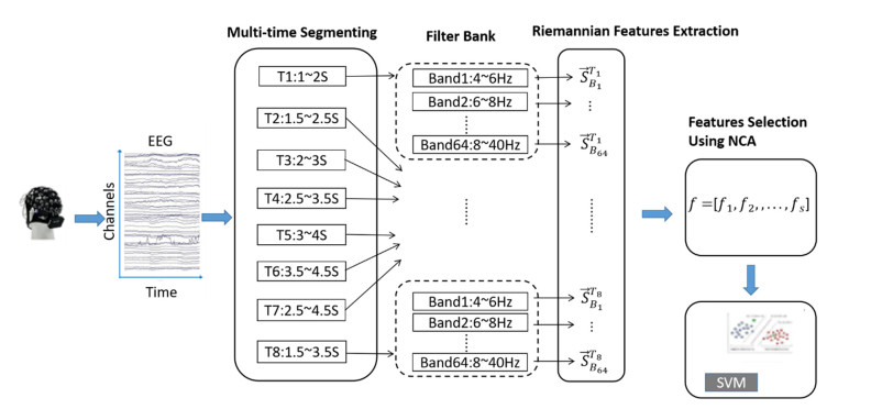
Motor imagery (MI) is a traditional paradigm of brain-computer interface (BCI) and can assist users in creating direct connections between their brains and external equipment. The common spatial patterns algorithm is the most popular spatial filtering technique for collecting EEG signal features in MI-based BCI systems. Due to the defect that it only considers the spatial information of EEG signals and is susceptible to noise interference and other issues, its performance is diminished. In this study, we developed a Riemannian transform feature extraction method based on filter bank fusion with a combination of multiple time windows. First, we proposed the multi-time window data segmentation and recombination method by combining it with a filter group to create new data samples. This approach could capture individual differences due to the variation in time-frequency patterns across different participants, thereby improving the model's generalization performance. Second, Riemannian geometry was used for feature extraction from non-Euclidean structured EEG data. Then, considering the non-Gaussian distribution of EEG signals, the neighborhood component analysis (NCA) algorithm was chosen for feature selection. Finally, to meet real-time requirements and a low complexity, we employed a Support Vector Machine (SVM) as the classification algorithm. The proposed model achieved improved accuracy and robustness. In this study, we proposed an algorithm with superior performance on the BCI Competition IV dataset 2a, achieving an accuracy of 89%, a kappa value of 0.73 and an AUC of 0.9, demonstrating advanced capabilities. Furthermore, we analyzed data collected in our laboratory, and the proposed method achieved an accuracy of 77.4%, surpassing other comparative models. This method not only significantly improved the classification accuracy of motor imagery EEG signals but also bore significant implications for applications in the fields of brain-computer interfaces and neural engineering.
Citation: Xiaotong Ding, Lei Yang, Congsheng Li. Study of MI-BCI classification method based on the Riemannian transform of personalized EEG spatiotemporal features[J]. Mathematical Biosciences and Engineering, 2023, 20(7): 12454-12471. doi: 10.3934/mbe.2023554
Motor imagery (MI) is a traditional paradigm of brain-computer interface (BCI) and can assist users in creating direct connections between their brains and external equipment. The common spatial patterns algorithm is the most popular spatial filtering technique for collecting EEG signal features in MI-based BCI systems. Due to the defect that it only considers the spatial information of EEG signals and is susceptible to noise interference and other issues, its performance is diminished. In this study, we developed a Riemannian transform feature extraction method based on filter bank fusion with a combination of multiple time windows. First, we proposed the multi-time window data segmentation and recombination method by combining it with a filter group to create new data samples. This approach could capture individual differences due to the variation in time-frequency patterns across different participants, thereby improving the model's generalization performance. Second, Riemannian geometry was used for feature extraction from non-Euclidean structured EEG data. Then, considering the non-Gaussian distribution of EEG signals, the neighborhood component analysis (NCA) algorithm was chosen for feature selection. Finally, to meet real-time requirements and a low complexity, we employed a Support Vector Machine (SVM) as the classification algorithm. The proposed model achieved improved accuracy and robustness. In this study, we proposed an algorithm with superior performance on the BCI Competition IV dataset 2a, achieving an accuracy of 89%, a kappa value of 0.73 and an AUC of 0.9, demonstrating advanced capabilities. Furthermore, we analyzed data collected in our laboratory, and the proposed method achieved an accuracy of 77.4%, surpassing other comparative models. This method not only significantly improved the classification accuracy of motor imagery EEG signals but also bore significant implications for applications in the fields of brain-computer interfaces and neural engineering.

| [1] | W. G. Zhang, L. Lu, A. N. Belkacem, J. X. Zhang, P. H. Li, J. Liang, et al., Classification of EEG signals based on GA-ELM optimization algorithm, in Human Brain and Artificial Intelligence (eds. X. M. Ying), HBAI, 1692 (2022), 3-14. https://doi.org/10.1007/978-981-19-8222-4_1 |
| [2] |
R. Sharma, M. Kim, A. Gupta, Motor imagery classification in brain-machine interface with machine learning algorithms: classical approach to multi-layer perceptron model, Biomed. Signal Process. Control, 71 (2022), 103101. https://doi.org/10.1016/j.bspc.2021.103101 doi: 10.1016/j.bspc.2021.103101

|
| [3] |
W. S. Pritchard, Psychophysiology of P300, Psychol. Bull., 89 (1981), 506-540. https://doi.org/10.1037/0033-2909.89.3.506 doi: 10.1037/0033-2909.89.3.506
|
| [4] |
A. M. Norcia, L. G. Appelbaum, J. M. Ales, B. R. Cottereau, B. Rossion, The steady-state visual evoked potential in vision research: a review, J. Vision, 15 (2015), 4. https://doi.org/10.1167/15.6.4 doi: 10.1167/15.6.4
|
| [5] |
G. Pfurtscheller, G. R. Muller-Putz, R. Scherer, C. Neuper, Rehabilitation with brain-computer interface systems, Computer, 41 (2008), 58-65. https://doi.org/10.1109/MC.2008.432 doi: 10.1109/MC.2008.432
|
| [6] |
C. Neuper, R. Scherer, M. Reiner, G. Pfurtscheller, Imagery of motor actions: differential effects of kinesthetic and visual-motor mode of imagery in single-trial EEG, Cognit. Brain Res., 25 (2005), 668-677. https://doi.org/10.1016/j.cogbrainres.2005.08.014 doi: 10.1016/j.cogbrainres.2005.08.014
|
| [7] |
F. Lotte, L. Bougrain, A. Cichocki, M. Clerc, M. Congedo, A. Rakotomamonjy, et al., A review of classification algorithms for EEG-based brain-computer interfaces: a 10-year update, J. Neural Eng., 15 (2018), 031005. https://doi.org/10.1088/1741-2552/aab2f2 doi: 10.1088/1741-2552/aab2f2
|
| [8] |
U. Talukdar, S. M. Hazarika, J. Q. Gan, Adaptive feature extraction in EEG-based motor imagery BCI: tracking mental fatigue, J. Neural Eng., 17 (2020). https://doi.org/10.1088/1741-2552/ab53f1 doi: 10.1088/1741-2552/ab53f1
|
| [9] |
F. Lotte, C. T. Guan, Regularizing common spatial patterns to improve BCI designs: unified theory and new algorithms, IEEE Trans. Biomed. Eng., 58 (2011), 355-362. https://doi.org/10.1109/TBME.2010.2082539 doi: 10.1109/TBME.2010.2082539
|
| [10] |
J. Jiang, C. H. Wang, J. H. Wu, W. Qin, M. P. Xu, E. W. Yin, Temporal combination pattern optimization based on feature selection method for motor imagery BCIs, Front. Hum. Neurosci., 14 (2020), 231. https://doi.org/10.3389/fnhum.2020.00231 doi: 10.3389/fnhum.2020.00231
|
| [11] | K. K. Ang, Z. Y. Chin, H. H. Zhang, C. T. Guan, Filter bank common spatial pattern (FBCSP) in brain-computer interface, in IEEE International Joint Conference on Neural Networks, 2008. https://doi.org/10.1109/IJCNN.2008.4634130 |
| [12] | K. P. Thomas, C. T. Guan, L. C. Tong, V. A. Prasad, An adaptive filter bank for motor imagery based brain computer interface, in International Conference of the IEEE Engi-neering in Medicine & Biology Society, Vancouver, BC, Canada, 2008. https://doi.org/10.1109/IEMBS.2008.4649353 |
| [13] |
A. Barachant, S. Bonnet, M. Congedo, C. Jutten, Multiclass brain–computer interface classification by Riemannian geometry, IEEE Trans. Biomed. Eng., 59 (2012), 920-928. https://doi.org/10.1109/TBME.2011.2172210 doi: 10.1109/TBME.2011.2172210
|
| [14] | A. Barachant, S. Bonnet, M. Congedo, C. Jutten, Common spatial pattem revisited by Riemannian geometry, in Proceedings of the 2010 IEEE International Workshop on Multimedi a Signal Processing, (2010), 472-476. https://doi.org/10.1109/MMSP.2010.5662067 |
| [15] | C. H. Nguyen, P. Artemiadis, EEG feature descriptors and discriminant analysis under Riemannian manifold perspective, Neurocomputing, 275 (2018). https://doi.org/10.1016/j.neucom.2017.10.013 |
| [16] |
H. Abdi, L. J. Williams, Principal component analysis, WIREs Comput. Stat., 2 (2010), 433-459. https://doi.org/10.1002/wics.101 doi: 10.1002/wics.101
|
| [17] |
J. Shao, Y. Z. Wang, X. W. Deng, S. J. Wang, Sparse linear discriminant analysis by thresholding for high dimensional data, Ann. Stat., 39 (2011), 1241-1265. https://doi.org/10.1214/10-AOS870 doi: 10.1214/10-AOS870
|
| [18] | Z. Q. Miao, X. Zhang, M. R. Zhao, D. Ming, LMDA-Net: a lightweight multi-dimensional attention network for general EEG-based brain-computer interface paradigms and interpretability, preprint, arXiv: 2303.16407. |
| [19] |
C. Neuper, G. Pfurtscheller, Evidence for distinct beta resonance frequencies in human EEG related to specific sensorimotor cortical areas, Clin. Neurophysiol., 112 (2001), 2084-2097. https://doi.org/10.1016/S1388-2457(01)00661-7 doi: 10.1016/S1388-2457(01)00661-7
|
| [20] |
O. Tuzel, F. Porikli, P. Meer, Pedestrian detection via classification on Riemannian manifolds, IEEE Trans. Pattern Anal. Mach. Intell., 30 (2008), 1713-1727. https://doi.org/10.1109/TPAMI.2008.75 doi: 10.1109/TPAMI.2008.75
|
| [21] |
M. Moakher, A differential geometric approach to the geometric mean of symmetric positive-definite matrices, SIAM J. Matrix Anal. Appl., 26 (2005), 735-747. https://doi.org/10.1137/S0895479803436937 doi: 10.1137/S0895479803436937
|
| [22] | P. T. Fletcher, S. Joshi, Principal geodesic analysis on symmetric spaces: statistics of diffusion tensors, in Computer Vision and Mathematical Methods in Medical and Biomedical Image Analysis, (2004), 87-98. https://doi.org/10.1007/978-3-540-27816-0_8 |
| [23] |
A. Barachant, S. Bonnet, M. Congedo, C. Jutten, Classification of covariance matrices using a Riemannian-based kernel for BCI applications, Neurocomputing, 112 (2013), 172-178. https://doi.org/10.1016/j.neucom.2012.12.039 doi: 10.1016/j.neucom.2012.12.039
|
| [24] | J. Goldberger, S. T. Roweis, G. E. Hinton, R. R. Salakhutdinov, Neighbourhood components analysis, in Proceedings of the 17th International Conference on Neural Information Processing Systems, Vancouver British Columbia Canada, (2004), 513-520. Available from: https://proceedings.neurips.cc/paper/2004/file/42fe880812925e520249e808937738d2-Paper.pdf. |
| [25] | H. Y. Sun, Y. Xiang, Y. R. Sun, H. P. Zhu, J. H. Zeng, On-line EEG classification for brain-computer interface based on CSP and SVM, in 2010 3rd International Congress on Image and Signal Processing, (2010), 4105-4108. https://doi.org/10.1109/CISP.2010.5648081 |
| [26] |
I. Syarif, A. Prugel-Bennett, G. Wills, SVM parameter optimization using grid search and genetic algorithm to improve classification performance, TELKOMNIKA, 14 (2016), 1502-1509. http://doi.org/10.12928/telkomnika.v14i4.3956 doi: 10.12928/telkomnika.v14i4.3956
|
| [27] |
K. K. Ang, Z. Y. Chin, C. C. Wang, C. T. Guan, H. H. Zhang, Filter bank common spatial pattern algorithm on BCI competition IV datasets 2a and 2b, Front. Neurosci., 6 (2012), 39. https://doi.org/10.3389/fnins.2012.00039 doi: 10.3389/fnins.2012.00039
|
| [28] |
Y. R. Tabar, U. Halici, A novel deep learning approach for classification of EEG motor imagery signals, J. Neural Eng., 14 (2017), 016003. https://doi.org/10.1088/1741-2560/14/1/016003 doi: 10.1088/1741-2560/14/1/016003
|
| [29] | J. Carletta, Assessing agreement on classification tasks: the Kappa statistic, Comput. Ling., 22 (1996), 249-254. Available from: https://aclanthology.org/J96-2004.pdf. |
| [30] | Y. Y. Miao, J. Jin, I. Daly, C. Zuo, X. Y. Wang, A. Cichocki, et al., Learning common time-frequency-spatial patterns for motor imagery classification, IEEE Trans. Neural Syst. Rehabil. Eng., 29 (2021), 699-707. https://doi.org/0.1109/TNSRE.2021.3071140 |
| [31] | K. Raj, A. Singh, A. Mandal, T. Kumar, A. M. Roy, Understanding EEG signals for subject-wise Definition of Armoni Activities, preprint, arXiv: 2301.00948. |
| [32] |
B. Jiang, S. Chen, B. B. Wang, B. Luo, MGLNN: semi-supervised learning via multiple graph cooperative learning neural networks, Neural Networks, 153 (2022), 204-214. https://doi.org/10.1016/j.neunet.2022.05.024 doi: 10.1016/j.neunet.2022.05.024
|


Figures(7) / Tables(3)

Xiaotong Ding, Lei Yang, Congsheng Li. Study of MI-BCI classification method based on the Riemannian transform of personalized EEG spatiotemporal features[J]. Mathematical Biosciences and Engineering, 2023, 20(7): 12454-12471. doi: 10.3934/mbe.2023554


 DownLoad: