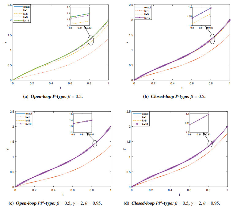
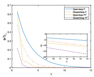
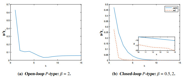
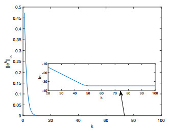
In this paper, the iterative learning control technique is extended to distributed parameter systems governed by nonlinear fractional diffusion equations. Based on $ P $-type and $ PI^{\theta} $-type iterative learning control methods, sufficient conditions for the convergences of systems are given. Finally, numerical examples are presented to illustrate the efficiency of the proposed iterative schemes. The numerical results show that the closed-loop iterative learning control scheme converges faster than the open-loop iterative learning control scheme and the $ PI^{\theta} $-type iterative learning control scheme converges faster than the $ P $-type and the $ PI $-type iterative learning control scheme.
Citation: Jungang Wang, Qingyang Si, Jun Bao, Qian Wang. Iterative learning algorithms for boundary tracing problems of nonlinear fractional diffusion equations[J]. Networks and Heterogeneous Media, 2023, 18(3): 1355-1377. doi: 10.3934/nhm.2023059
In this paper, the iterative learning control technique is extended to distributed parameter systems governed by nonlinear fractional diffusion equations. Based on $ P $-type and $ PI^{\theta} $-type iterative learning control methods, sufficient conditions for the convergences of systems are given. Finally, numerical examples are presented to illustrate the efficiency of the proposed iterative schemes. The numerical results show that the closed-loop iterative learning control scheme converges faster than the open-loop iterative learning control scheme and the $ PI^{\theta} $-type iterative learning control scheme converges faster than the $ P $-type and the $ PI $-type iterative learning control scheme.

| [1] |
S. Arimoto, S. Kawamura, F. Miyazaki, Bettering operation of robots by learning, J. Robot. Syst., 1 (1984), 123–140. https://doi.org/10.1002/rob.4620010203 doi: 10.1002/rob.4620010203

|
| [2] | Z. Chen, H. Wu, Selected Topics in Finite Element Methods, Beijing: Science Press, 2010. |
| [3] |
J. Choi, B. Seo, K. Lee, Constrained digital regulation of hyperbolic pde systems: A learning control approach, Korean J. Chem. Eng., 18 (2001), 606–611. https://doi.org/10.1007/BF02706375 doi: 10.1007/BF02706375
|
| [4] |
J. Craig, Adaptive control of manipulators through repeated trials, Am. Control Conf., 21 (1984), 1566–1573. http://dx.doi.org/10.1109/ACC.1984.4171549 doi: 10.1109/ACC.1984.4171549
|
| [5] |
X. Dai, S. Tian, Y. Peng, W. Luo, Closed-loop P-type iterative learning control of uncertain linear distributed parameter systems, IEEE/CAA J. Automatica Sinica, 1 (2014), 267–273. https://doi.org/10.1109/JAS.2014.7004684 doi: 10.1109/JAS.2014.7004684
|
| [6] |
S. Das, I. Pan, S. Das, A. Gupta, Improved model reduction and tuning of fractional-order $PI^\lambda$D$^\mu$ controllers for analytical rule extraction with genetic programming, ISA Trans., 51 (2012), 237–261. https://doi.org/10.1016/j.isatra.2011.10.004 doi: 10.1016/j.isatra.2011.10.004
|
| [7] |
M. A. Duarte-Mermoud, N. Aguila-Camacho, J. A. Gallegos, R. Castro-Linares, Using general quadratic lyapunov functions to prove lyapunov uniform stability for fractional order systems, Commun. Nonlinear Sci., 22 (2015), 650–659. https://doi.org/10.1016/j.cnsns.2014.10.008 doi: 10.1016/j.cnsns.2014.10.008
|
| [8] | M. Garden, Learning Control of Actuators in Control Systems, Washington, DC: US Patent, 1971. |
| [9] |
K. Hamamoto, T. Sugie, Iterative learning control for robot manipulators using the finite dimensional input subspace, IEEE Trans. Robot. Autom., 18 (2002), 632–635. https://doi.org/10.1109/TRA.2002.801050 doi: 10.1109/TRA.2002.801050
|
| [10] |
Z. Hou, J. Xu, J. Yan, An iterative learning approach for density control of freeway traffic flow via ramp metering, Transp. Res. Part C Emerg. Technol., 16 (2008), 71–97. https://doi.org/10.1016/j.trc.2007.06.007 doi: 10.1016/j.trc.2007.06.007
|
| [11] |
C. Huang, J. Cao, Active control strategy for synchronization and anti-synchronization of a fractional chaotic financial system, Physica A, 473 (2017), 262–275. https://doi.org/10.1016/j.physa.2017.01.009 doi: 10.1016/j.physa.2017.01.009
|
| [12] |
D. Huang, X. Li, W. He, S. Zhang, Iterative learning control for boundary tracking of uncertain nonlinear wave equations, J. Franklin Inst., 355 (2018), 8441–8461. https://doi.org/10.1016/j.jfranklin.2018.10.004 doi: 10.1016/j.jfranklin.2018.10.004
|
| [13] |
D. Huang, J. Xu, X. Li, C. Xu, M. Yu, D-type anticipatory iterative learning control for a class of inhomogeneous heat equations, Automatica, 49 (2013), 2397–2408. https://doi.org/10.1016/j.automatica.2013.05.005 doi: 10.1016/j.automatica.2013.05.005
|
| [14] |
X. Jin, Adaptive iterative learning control for high-order nonlinear multi-agent systems consensus tracking, Syst. Control Lett., 89 (2016), 16–23. https://doi.org/10.1016/j.sysconle.2015.12.009 doi: 10.1016/j.sysconle.2015.12.009
|
| [15] | J. Kang, A newton-type iterative learning algorithm of output tracking control for uncertain nonlinear distributed parameter systems, in Proceedings of the 33rd Chinese Control Conference, IEEE, Nanjing, (2014), 8901–8905. https://doi.org/10.1109/ChiCC.2014.6896498 |
| [16] | S. Kawamura, Iterative learning control for robotic systems, Proc. IECON'84, (1984), 393–398. |
| [17] | A. A. Kilbas, H. M. Srivastava, J. J. Trujillo, Theory and Applications of Fractional Differential Equations, USA: Elsevier, 204 (2006), 540. |
| [18] | H. Kinateder, N. F. Wagner, Multiple-period market risk prediction under long memory: When var is higher than expected, J. Risk Finance, 15 (2014), 4–32. |
| [19] |
Y. H. Lan, W. Bin, Y. Zhou, Iterative learning consensus control with initial state learning for fractional order distributed parameter models multi-agent systems, Math. Methods Appl. Sci., 45 (2022), 5–20. https://doi.org/10.1002/mma.7589 doi: 10.1002/mma.7589
|
| [20] | Y. Lan, L. Lin, J. Xia, P-type iterative learning control for a class of fractional order distributed parameter switched systems, in 2018 37th Chinese Control Conference (CCC), IEEE, Wuhan, (2018), 2836–2841. https://doi.org/10.23919/ChiCC.2018.8483310 |
| [21] |
Y. H. Lan, L. Liu, Y. P. Luo, Iterative learning control for a class of fractional order distributed parameter systems, Asian J. Control, 22 (2020), 449–459. https://doi.org/10.1002/asjc.1908 doi: 10.1002/asjc.1908
|
| [22] |
Y. Lan, B. Wu, Y. Shi, Y. Luo, Iterative learning based consensus control for distributed parameter multi-agent systems with time-delay, Neurocomputing, 357 (2019), 77–85. https://doi.org/10.1016/j.neucom.2019.04.064 doi: 10.1016/j.neucom.2019.04.064
|
| [23] |
S. Liu, J. Wang, W. Wei, A study on iterative learning control for impulsive differential equations, Commun. Nonlinear Sci. Numer. Simul., 24 (2015), 4–10. https://doi.org/10.1016/j.cnsns.2014.12.002 doi: 10.1016/j.cnsns.2014.12.002
|
| [24] |
D. Luo, J. Wang, D. Shen, Learning formation control for fractional-order multiagent systems, Math. Methods Appl. Sci., 41 (2018), 5003–5014. https://doi.org/10.1002/mma.4948 doi: 10.1002/mma.4948
|
| [25] |
D. Luo, J. Wang, D. Shen, $PD^{\alpha}$‐type distributed learning control for nonlinear fractional‐order multiagent systems, Math. Methods Appl. Sci., 42 (2019), 4543–4553. https://doi.org/10.1002/mma.5677 doi: 10.1002/mma.5677
|
| [26] |
F. Memon, C. Shao, An optimal approach to online tuning method for pid type iterative learning control, Int. J. Control Autom. Syst., 18 (2020), 1926–1935. https://doi.org/10.1007/s12555-018-0840-0 doi: 10.1007/s12555-018-0840-0
|
| [27] | I. Podlubny, Fractional Differential Equations, Mathematics in Science and Engineering, New York: Academic press, 1999. |
| [28] |
M. Uchiyama, Formation of high-speed motion pattern of a mechanical arm by trial, Trans. Soc. Instrum. Control Eng., 14 (1978), 706–712. https://doi.org/10.9746/sicetr1965.14.706 doi: 10.9746/sicetr1965.14.706
|
| [29] |
X. Wang, J. Wang, D. Shen, Y. Zhou, Convergence analysis for iterative learning control of conformable fractional differential equations, Math. Methods Appl. Sci., 41 (2018), 8315–8328. https://doi.org/10.1002/mma.5291 doi: 10.1002/mma.5291
|
| [30] | C. Xu, R. Arastoo, E. Schuster, On iterative learning control of parabolic distributed parameter systems, in 2009 17th Mediterranean Conference on Control and Automation, IEEE, Thessaloniki, Greece, (2017), 510–515. https://doi.org/10.1109/MED.2009.5164593 |
| [31] |
H. Ye, J. Gao, Y. Ding, A generalized gronwall inequality and its application to a fractional differential equation, J. Math. Anal. Appl., 328 (2007), 1075–1081. https://doi.org/10.1016/j.jmaa.2006.05.061 doi: 10.1016/j.jmaa.2006.05.061
|
| [32] |
J. Zhang, B. Cui, Z. Jiang, J. Chen, A pd-type iterative learning algorithm for semi-linear distributed parameter systems with sensors/actuators, IEEE Access 7 (2019), 159037–159047. https://doi.org/10.1109/ACCESS.2019.2950456 doi: 10.1109/ACCESS.2019.2950456
|
Figures(4) / Tables(2)
Jungang Wang, Qingyang Si, Jun Bao, Qian Wang. Iterative learning algorithms for boundary tracing problems of nonlinear fractional diffusion equations[J]. Networks and Heterogeneous Media, 2023, 18(3): 1355-1377. doi: 10.3934/nhm.2023059


 DownLoad: