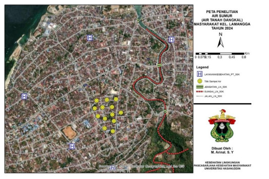
High concentrations of detergent waste disrupt aquatic biota. Detergent content can increase nutrient levels, causing environmental problems. The purpose of this study was to determine the level of public health risk in Lamangga Village, Baubau City, where well water containing phosphate and surfactants is consumed. This was an observational study with environmental health risk analysis. The study was composed of representative samples from 14 wells used as a source of drinking water and 70 respondents. The results showed that the average concentration of phosphate in drinking water sources across the 14 sampling points was 0.020 mg/L and that of surfactants was 0.39 mg/L. The rate of exposure to detergent concentration in raw water (intake rate) is directly proportional to the risk level value (RQ). The RQ of all respondents was ≤ 1. All 70 respondents had a target hazard quotient (THQ) ≤ 1, and no respondents had a THQ value higher than 1. The standardization values issued by the US-EPA Agency and the Regulation of the Minister of Health of the Republic of Indonesia Number 32/2017 set the reference dose (RfD) value of surfactants and phosphate at 0.05 mL/L/d. Surfactant exposure can cause irritation to the skin and eyes and damage the skin's natural protective layer, while phosphate exposure is not directly toxic to humans in small concentrations. Risk management strategies are necessary to control phosphate and surfactant concentrations in drinking water so that they do not result in future non-carcinogenic risk effects.
Citation: Muhammad Arinal Surgama Yusuf, Anwar Mallongi, Anwar Daud, Agus Bintara Birawida, Sukri Palutturi, Lalu Muhammad Saleh, Setiawan Kasim. Environmental health risk analysis from detergent contamination in well water[J]. AIMS Environmental Science, 2025, 12(2): 256-275. doi: 10.3934/environsci.2025013
High concentrations of detergent waste disrupt aquatic biota. Detergent content can increase nutrient levels, causing environmental problems. The purpose of this study was to determine the level of public health risk in Lamangga Village, Baubau City, where well water containing phosphate and surfactants is consumed. This was an observational study with environmental health risk analysis. The study was composed of representative samples from 14 wells used as a source of drinking water and 70 respondents. The results showed that the average concentration of phosphate in drinking water sources across the 14 sampling points was 0.020 mg/L and that of surfactants was 0.39 mg/L. The rate of exposure to detergent concentration in raw water (intake rate) is directly proportional to the risk level value (RQ). The RQ of all respondents was ≤ 1. All 70 respondents had a target hazard quotient (THQ) ≤ 1, and no respondents had a THQ value higher than 1. The standardization values issued by the US-EPA Agency and the Regulation of the Minister of Health of the Republic of Indonesia Number 32/2017 set the reference dose (RfD) value of surfactants and phosphate at 0.05 mL/L/d. Surfactant exposure can cause irritation to the skin and eyes and damage the skin's natural protective layer, while phosphate exposure is not directly toxic to humans in small concentrations. Risk management strategies are necessary to control phosphate and surfactant concentrations in drinking water so that they do not result in future non-carcinogenic risk effects.

| [1] |
Anand AJ, ChuaMC, Khoo SH, et al. (2017) Early discharge planning in preterm low birth weight babies: A quality improvement project. Proc Singap Healthc 26: 98–101. https://doi.org/10.1177/2010105816676827 doi: 10.1177/2010105816676827

|
| [2] |
Lestari AD (2022) Pengaruh pencemaran limbah detergen terhadap ekosistem perairan. Jurnal Sains Indonesia 3: 24–36. https://doi.org/10.59897/jsi.v3i1.72 doi: 10.59897/jsi.v3i1.72
|
| [3] |
Naufal BS, A'yun DQ (2024) Analisis dampak pencemaran tanah akibat limbah deterjen terhadap lingkungan hidup masyarakat di daerah pedesaan. Stud Res J 2: 231–235. https://doi.org/10.55606/srjyappi.v2i3.1320 doi: 10.55606/srjyappi.v2i3.1320
|
| [4] |
Apriyani N (2017) Reduction of surfactant and sulfate levels in laundry waste. Environ Eng Sci Media 2: 37–44. https://doi.org/10.33084/mitl.v2i1.132 doi: 10.33084/mitl.v2i1.132
|
| [5] | Al Kholif M (2020) Domestic waste processing, Scopindo: Media Pustaka. |
| [6] |
Sulistia S, Septisya AC (2020) Analysis of domestic office wastewater quality. J Environ Eng 12: 41–57. https://doi.org/10.29122/jrl.v12i1.3658 doi: 10.29122/jrl.v12i1.3658
|
| [7] |
Pungut P, Al Kholif M, Pratiwi WDI (2021) Reduction of chemical oxygen demand (COD) and phosphate levels in laundry waste using adsorption method. J Environ Sci Te 13: 155–165. https://doi.org/10.20885/jstl.vol13.iss2.art6 doi: 10.20885/jstl.vol13.iss2.art6
|
| [8] |
Mukherjee S, Edmunds MBS, Lei X, et al. (2010) Steric acid delivery to corneum from a mild and moisturizing cleanser. J Cosmet Dermatol 3: 202–210. https://doi.org/10.1111/j.1473-2165.2010.00510.x doi: 10.1111/j.1473-2165.2010.00510.x
|
| [9] | Effendi H (2003) Water quality assessment: For aquatic resources and environmental management, Kanisius. |
| [10] |
Nurrosyidah IH, Putri EN, Klau ICS, et al. (2023) Formulasi Deterjen Eco-Friendly Ekstrak Etanol Biji Buah Lerak (Sapindus rarak DC) Kombinasi Surfaktan Decyl Glucoside dan Lauryl Glucoside. Clin Pharm Anal Pharm Community J 2: 84–91. https://doi.org/10.30651/cam.v2i1.17955 doi: 10.30651/cam.v2i1.17955
|
| [11] |
Saleh R, Daud A, Ishak H, et al. (2023) Spatial distribution of microplastic contamination in blood clams (Anadara granosa) on the Jeneponto coast, South Sulawesi. Pharm J 15: 680–690. https://doi.org/10.5530/pj.2023.15.137 doi: 10.5530/pj.2023.15.137
|
| [12] |
Suryana T, Makhroji M, Suryani S (2024) Pembuatan Detergen Ekonomis dan Ramah Lingkungan untuk Meningkatkan Pengetahuan Ibu PKK di Desa Karangbenda. Jurnal Kreativitas Pengabdian Kepada Masyarakat 7: 530–540. https://doi.org/10.38204/darmaabdikarya.v3i2.2154 doi: 10.38204/darmaabdikarya.v3i2.2154
|
| [13] | Subhan M, Birawida AB, Hatta M (2020) Health risk analysis of detergent concentration in raw water for drinking water on the community in Barrang Lompo Island, Makassar City. J Akademika 17: 25–30. |
| [14] | Wulandari N, Perwira IY, Ernawati NM (2021) Phosphate content profile in water in the Tukad Ayung River Basin (DAS), Bali. Jurnal Harian Regional 115: 108–115. Available from: https://jurnal.harianregional.com/ctas/id-59708. |
| [15] |
Manurung MB, Edhi T, Soesilo B, et al. (2022) Health risk analysis of detergent contamination in communities on Kodingareng Lompo Island, Makassar City. Journal Presipitasi 19: 426–435. https://doi.org/10.14710/presipitasi.v19i2.426–435 doi: 10.14710/presipitasi.v19i2.426–435
|
| [16] |
Birawida AB, Ibrahim E, Mallongi A, et al. (2021) Clean water supply vulnerability model for improving the quality of public health (environmental health perspective): A case in Spermonde islands, Makassar Indonesia. Gac Sanit 35: S601–S603. https://doi.org/10.1016/j.gaceta.2021.10.095 doi: 10.1016/j.gaceta.2021.10.095
|
| [17] | Putri BH, Kurniawan A, Pi S (2021) Kajian Literatur Aplikasi Bakteri Dalam Mendegradasi Surfaktan di Lingkungan Perairan, Diss. Universitas Brawijaya. |
| [18] |
Kasim S, Daud A, Birawida AB, et al. (2023) Analysis of environmental health risks from exposure to polyethylene terephthalate microplastics in refilled drinking. Glob J Environ Sci M 9: 301–318. https://doi.org/10.22034/GJESM.2023.09.SI.17 doi: 10.22034/GJESM.2023.09.SI.17
|
| [19] |
Hidayat H, La Taha LT, Dewi BS (2022) Risk analysis of lead (Pb) exposure in shellfish in the coastal area of Galesong Village, Palalakkang District, Galesong Regency, Takalar Regency. Sulolipu Media Commun Acad Community 22: 219–225. https://doi.org/10.32382/sulolipu.v22i2.2902 doi: 10.32382/sulolipu.v22i2.2902
|
| [20] | Dirjen P2PL (2012) Guidance on environmental health risk analysis. |
| [21] |
Diyanah KCS (2022) Risk analysis of dust exposure (total suspended particulate) in Packer Unit PT. X. Environ Health J 9: 100–110. https://doi.org/10.20473/jkl.v9i1.2017.100-101 doi: 10.20473/jkl.v9i1.2017.100-101
|
| [22] | Badamasi H, Yaro MN, Ibrahim A, et al. (2019) Impacts of phosphates on water quality and aquatic life. Chem Res J 4: 124–133. Available from: https://chemrj.org/download/vol-4-iss-3-2019/chemrj-2019-04-03-124-133.pdf. |
| [23] |
Sutamihardja R, Azizah M, Hardini Y (2018) Study of phosphate compound dynamics in the water quality of the upper Ciliwung River in Bogor City. J Nat Sci 8: 43–49. https://doi.org/10.31938/jsn.v8i1.114 doi: 10.31938/jsn.v8i1.114
|
| [24] | Fajriah N, Alawiyah T, Wusko IU (2020) Analysis of anionic surfactant levels (detergents) in Barito River water using visible spectrophotometry method. J Pharm Care Sci 1: 55–61. Available from: https://ejurnal.unism.ac.id/index.php/jpcs/article/view/22. |
| [25] |
Larasati NN, Wulandari SY, Maslukah L, et al. (2021) Detergent pollutant content and water quality in the Tapak River Estuary, Semarang. Indones J Oceanography 3: 22–29. https://doi.org/10.14710/ijoce.v3i1.9470 doi: 10.14710/ijoce.v3i1.9470
|
| [26] |
Invally K, Ju L (2017) Biolytic effect of rhamnolipid biosurfactant and dodecyl sulfate against phagotrophic alga Ochromonas danica. J Surfactants Deterg 20: 1161–1171. https://doi.org/10.1007/s11743-017-2005-1 doi: 10.1007/s11743-017-2005-1
|
| [27] |
Colonna WJ, Martí ME, Nyman JA, et al. (2016). Hemolysis as a rapid screening technique for assessing the toxicity of native surfactin and a genetically engineered derivative. Environ Prog Sustain 36: 505–510. https://doi.org/10.1002/ep.12444 doi: 10.1002/ep.12444
|
| [28] |
Ríos F, Lechuga M, Guarnido IL, et al. (2023) Antagonistic toxic effects of surfactants mixtures to Pseudomonas putida and marine microalgae Phaeodactylum tricornutum. Toxics 11: 344–350. https://doi.org/10.3390/toxics11040344 doi: 10.3390/toxics11040344
|
| [29] |
Martín PAL, Li X, Bopp RF, et al. (2010) Occurrence of alkyltrimethylammonium compounds in urban estuarine sediments: Behentrimonium as a new emerging contaminant. Environ Sci Tech 44: 7569–7575. https://doi.org/10.1021/es101169a doi: 10.1021/es101169a
|
| [30] |
García MT, Kaczerewska O, Ribosa I, et al. (2016) Biodegradability and aquatic toxicity of quaternary ammonium-based gemini surfactants: Effect of the spacer on their ecological properties. Chemosphere 154: 155–160. https://doi.org/10.1016/j.chemosphere.2016.03.109 doi: 10.1016/j.chemosphere.2016.03.109
|
| [31] |
Mesnage R, Antoniou M (2018) Ignoring adjuvant toxicity falsifies the safety profile of commercial pesticides. Front Public Health 5: 43–50. https://doi.org/10.3389/fpubh.2017.00361 doi: 10.3389/fpubh.2017.00361
|
| [32] |
Mikó Z, Hettyey A (2023) Toxicity of POEA-containing glyphosate-based herbicides to amphibians is mainly due to the surfactant, not to the active ingredient. Ecotoxicology 32: 150–159. https://doi.org/10.1007/s10646-023-02626-x doi: 10.1007/s10646-023-02626-x
|
| [33] |
Collins JK, Jackson JM (2022) Application of a screening-level pollinator risk assessment framework to trisiloxane polyether surfactants. Environ Toxicol Chem 41: 3084–3094. https://doi.org/10.1002/etc.5479 doi: 10.1002/etc.5479
|
| [34] |
Khamidulina Kh, Proskurina AS (2020) About measures to reduce the risk of cyanotoxins exposure to the health of population by regulating phosphates in synthetic detergents. Toxicol Rev 3: 3–8. https://doi.org/10.36946/0869-7922-2020-3-3-8 doi: 10.36946/0869-7922-2020-3-3-8
|
| [35] |
Badmus SO, Amusa HK, Oyehan TA (2021) Environmental risks and toxicity of surfactants: Overview of analysis, assessment, and remediation techniques. Environ Sci Pollut R 28: 62085–62104. https://doi.org/10.1007/s11356-021-16483-w doi: 10.1007/s11356-021-16483-w
|
| [36] | Anpilova Y, Yakovliev Y, Trofymchuk O, et al. (2021). Environmental hazards of the Donbas hydrosphere at the final stage of the coal mines flooding, In: Zaporozhets A. Eds., Systems, Decision and Control in Energy Ⅲ, Cham: Springer, 345–350. https://doi.org/10.1007/978-3-030-87675-3_19 |
| [37] |
Setiawan I, Bandung PN (2022) Development of a prototype of an ISO 31000-based risk management application. Matrix: J Tech Inform M 10: 26–33. https://doi.org/10.31940/matrix.v10i1.1817 doi: 10.31940/matrix.v10i1.1817
|
| [38] |
Yoewono JO, Prasetyo AH (2022) Design and risk management process at PT Surya Harmonica Cita. Estuary Econ Business J 6: 56–62. https://doi.org/10.24912/jmieb.v6i1.12207 doi: 10.24912/jmieb.v6i1.12207
|
| [39] |
Trimadya NM, Hardjomidjojo H, Anggraeni E (2018) Contamination risk management system in the food supply chain (case study: pasteurized milk). J Agric Ind Technol 28: 162–170. https://doi.org/10.24961/j.tek.ind.pert.2018.28.2.162 doi: 10.24961/j.tek.ind.pert.2018.28.2.162
|
| [40] |
Hisprastin Y, Musfiroh I (2020) Ishikawa diagram and failure mode effect analysis (FMEA) as methods frequently used in quality risk management in industry. Farmasetika Magazine 6: 1–10. https://doi.org/10.24198/mfarmasetika.v6i1.27106 doi: 10.24198/mfarmasetika.v6i1.27106
|
| [41] |
Fachrezi MI (2021) Information technology asset security risk management using ISO 31000:2018 Salatiga City Communication and Information Service. J Inform Eng Inform Syst 8: 764–773. https://doi.org/10.35957/jatisi.v8i2.789 doi: 10.35957/jatisi.v8i2.789
|
| [42] |
Wardoyo DU, Ramdhani ND, Ramadhan R (2022) The influence of solvency, institutional ownership, and independent commissioners on risk management disclosure. J-Ceki: Jurnal Cendekia Ilmiah 1: 57–64. https://doi.org/10.56799/jceki.v1i2.128 doi: 10.56799/jceki.v1i2.128
|
| [43] |
Mudrifah M, Wisyastuti A (2021) Strengthening the characteristics of human resources in the implementation of risk-based management at Lazis Muhammadiyah (Lazismu) Malang Regency. Indones National Serv J 2: 19–27. https://doi.org/10.35870/jpni.v2i1.26 doi: 10.35870/jpni.v2i1.26
|


Figures(6) / Tables(7)

Muhammad Arinal Surgama Yusuf, Anwar Mallongi, Anwar Daud, Agus Bintara Birawida, Sukri Palutturi, Lalu Muhammad Saleh, Setiawan Kasim. Environmental health risk analysis from detergent contamination in well water[J]. AIMS Environmental Science, 2025, 12(2): 256-275. doi: 10.3934/environsci.2025013


 DownLoad: