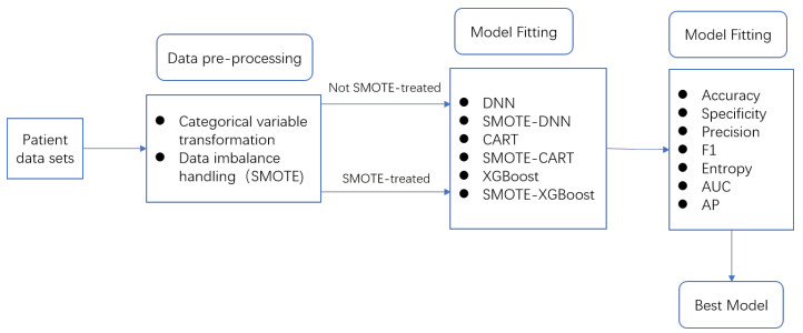
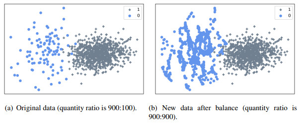
Prior to the surgical removal of an acoustic neuroma, the majority of patients anticipate that their hearing will be preserved to the greatest possible extent following surgery. This paper proposes a postoperative hearing preservation prediction model for the characteristics of class-imbalanced hospital real data based on the extreme gradient boost tree (XGBoost). In order to eliminate sample imbalance, the synthetic minority oversampling technique (SMOTE) is applied to increase the number of underclass samples in the data. Multiple machine learning models are also used for the accurate prediction of surgical hearing preservation in acoustic neuroma patients. In comparison to research results from existing literature, the experimental results found the model proposed in this paper to be superior. In summary, the method this paper proposes can make a significant contribution to the development of personalized preoperative diagnosis and treatment plans for patients, leading to effective judgment for the hearing retention of patients with acoustic neuroma following surgery, a simplified long medical treatment process and saved medical resources.
Citation: Cenyi Yang. Prediction of hearing preservation after acoustic neuroma surgery based on SMOTE-XGBoost[J]. Mathematical Biosciences and Engineering, 2023, 20(6): 10757-10772. doi: 10.3934/mbe.2023477
Prior to the surgical removal of an acoustic neuroma, the majority of patients anticipate that their hearing will be preserved to the greatest possible extent following surgery. This paper proposes a postoperative hearing preservation prediction model for the characteristics of class-imbalanced hospital real data based on the extreme gradient boost tree (XGBoost). In order to eliminate sample imbalance, the synthetic minority oversampling technique (SMOTE) is applied to increase the number of underclass samples in the data. Multiple machine learning models are also used for the accurate prediction of surgical hearing preservation in acoustic neuroma patients. In comparison to research results from existing literature, the experimental results found the model proposed in this paper to be superior. In summary, the method this paper proposes can make a significant contribution to the development of personalized preoperative diagnosis and treatment plans for patients, leading to effective judgment for the hearing retention of patients with acoustic neuroma following surgery, a simplified long medical treatment process and saved medical resources.

| [1] | M. Samii, Surgery of Cerebellopontine Lesions, Springer-Verlag Berlin Heidelberg, 2013. https://doi.org/10.1007/978-3-642-35422-9_5 |
| [2] |
E. S. Murphy, J. H. Suh, Radiotherapy for vestibular schwannomas: A critical review, Int. J. Radiat. Oncol. Biol. Phys., 79 (2011), 985–997. https://doi.org/10.1016/j.ijrobp.2010.10.010 doi: 10.1016/j.ijrobp.2010.10.010

|
| [3] |
M. Samii, V. M. Gerganov, A. Samii, Functional outcome after complete surgical removal of giant vestibular schwannomas, J. Neurosurg., 112 (2010), 860–867. https://doi.org/10.3171/2009.7.JNS0989 doi: 10.3171/2009.7.JNS0989
|
| [4] |
M. Samii, V. M. Gerganov, A. Samii, Quasi-morphisms and the Poisson bracket, J. Neurosurg., 40 (1997), 248–262. https://doi.org/10.1097/0006123-199701000-00001 doi: 10.1097/0006123-199701000-00001
|
| [5] |
S. Basu, K. T. Johnson, S. A. Berkowitz, Use of machine learning approaches in clinical epidemiological research of diabetes, Curr. Diab. Rep., 20 (2020), 80–99. https://doi.org/10.1007/s11892-020-01353-5 doi: 10.1007/s11892-020-01353-5
|
| [6] | J. Azmi, M. Arif, M. T. Nafis, M. A. Alam, S. Tanweer, G. Wang, A systematic review on machine learning approaches for cardiovascular disease prediction using medical big data, Med. Eng. Phys., 105 (2022), 103825. |
| [7] | K. Oliver, M. Stuart, B. Richard, Machine learning as a new horizon for colorectal cancer risk prediction? A systematic review, Health Sci. Rev., 105 (2022), 10041. |
| [8] |
O. W. Samuel, G. M. Asogbon, A. K. Sangaiah, P. Fang, G. Li, An integrated decision support system based on ANN and fuzzy-AHP for heart failure risk prediction, Expert Syst. Appl., 68 (2017), 163–172. https://doi.org/10.1016/j.eswa.2016.10.020 doi: 10.1016/j.eswa.2016.10.020
|
| [9] |
Z. Arabasadi, R. Alizadehsani, M. Roshanzamir, H. Moosaei, A. A. Yarifard, Computer aided decision making for heart disease detection using hybrid neural network-genetic algorithm, Comput. Methods Programs Biomed., 141 (2017), 19–26. https://doi.org/10.1016/j.cmpb.2017.01.004 doi: 10.1016/j.cmpb.2017.01.004
|
| [10] |
Y. J. King, M. Saqlian, J. Y. Lee, Deep learning-based prediction model of occurrences of major adverse cardiac events during 1-year follow-up after hospital discharge in patients with AMI using knowledge mining, Pers. Ubiquit. Comput., 26 (2022), 259–267. https://doi.org/10.1007/s00779-019-01248-7 doi: 10.1007/s00779-019-01248-7
|
| [11] |
S. W. A. Sherazi, J. Bae, J. Y. Lee, A soft voting ensemble classifier for early prediction and diagnosis of occurrences of major adverse cardiovascular event for STEMI and NSTEMI during 1-year follow-up in patients with acute coronary syndrome, PLoS One, 16 (2021), e0249338. https://doi.org/10.1371/journal.pone.0249338 doi: 10.1371/journal.pone.0249338
|
| [12] |
H. L. T. Lam, N. H. Le, L. van Tuan, H. T. Ban, T. N. K. Hung, N. T. K. Nguyen, et al., Machine learning model for identifying antioxidant proteins using features calculated from primary sequences, Biology (Basel), 9 (2020), 325. https://doi.org/10.3390/biology9100325 doi: 10.3390/biology9100325
|
| [13] |
T. H. Vo, N. T. K. Nguyen, Q. H. Kha, N. Q. K. Le, On the road to explainable AI in drug-drug interactions prediction: A systematic review, Comput. Struct. Biotechnol. J., 9 (2020), 325. https://doi.org/10.1016/j.csbj.2022.04.021 doi: 10.1016/j.csbj.2022.04.021
|
| [14] |
T. N. K. Hung, N. Q. K. Le, N. H. Le, L. van Tuan, T. P. Nguyen, C. Thi, et al., An AI-based prediction model for drug-drug interactions in osteoporosis and paget's diseases from SMILES, Mol. Inform., 9 (2020), 325. https://doi.org/10.1002/minf.202100264 doi: 10.1002/minf.202100264
|
| [15] |
N. Hafeez, X. Du, N. Boulgouris, P. Begg, R. Irving, C. Coulson, et al., Electrical impedance guides electrode array in cochlear implantation using machine learning and robotic feeder, Hear. Res., 412 (2021), 108371. https://doi.org/10.1016/j.heares.2021.108371 doi: 10.1016/j.heares.2021.108371
|
| [16] |
W. Duan, S. S. C. Congress, G. Cai, S. Liu, X. Dong, R. Chen, et al., A hybrid GMDH neural network and logistic regression framework for state parameter–based liquefaction evaluation, Can. Geotech. J., 58 (2021), 1801–1811. https://doi.org/10.1139/cgj-2020-0686 doi: 10.1139/cgj-2020-0686
|
| [17] |
J. Skidmore, L. Xu, X. Chao, W. J. Riggs, A. Pellittieri, C. Vaughan, et al., Prediction of the functional status of the cochlear nerve in individual cochlear implant users using machine learning and electrophysiological measures, Ear Hear., 42 (2021), 180-192. https://doi.org/10.1097/AUD.0000000000000916 doi: 10.1097/AUD.0000000000000916
|
| [18] |
W. Duan, Z. Zhao, G. Cai, S. Pu, S. Liu, X. Dong, Evaluating model uncertainty of an in situ state parameter-based simplified method for reliability analysis of liquefaction potential, Comput. Geotech., 151 (2022), 104957. https://doi.org/10.1016/j.compgeo.2022.104957 doi: 10.1016/j.compgeo.2022.104957
|
| [19] |
Y. Bozhkov, J. Shawarba, J. Feulner, F. Winter, S. Rampp, U. Hoppe, er al., Prediction of hearing preservation in vestibular schwannoma surgery according to tumor size and anatomic extension, Otolaryngol. Head Neck Surg., 166 (2021), 530–536. https://doi.org/10.1177/01945998211012674 doi: 10.1177/01945998211012674
|
| [20] |
J. H. Han, D. G. Kim, H. T. Chung, S. H. Paek, C. K. Park, Hearing preservation in patients with unilateral vestibular schwannoma who undergo stereotactic radiosurgery: Reinterpretation of the auditory brainstem response, Cancer, 118 (2012), 5441–5447. https://doi.org/10.1002/cncr.27501 doi: 10.1002/cncr.27501
|
| [21] |
A. Elliott, A. L. Hebb, S. Walling, D. P. Morris, M. Bance, Hearing preservation in vestibular schwannoma management, Am. J. Otolaryngol., 36 (2015), 526–534. https://doi.org/10.1016/j.amjoto.2015.02.016 doi: 10.1016/j.amjoto.2015.02.016
|
| [22] |
Y. Ren, K. O. Tawfik, B. J. Mastrodimos, R. A. Cueva, Preoperative radiographic predictors of hearing preservation after retrosigmoid resection of vestibular schwannomas, Otolaryngol. Head Neck Surg., 165 (2021), 344–353. https://doi.org/10.1177/0194599820978246 doi: 10.1177/0194599820978246
|
| [23] |
D. E. Roos, A. E. Potter, A. C. Zacest, Hearing preservation after low dose linac radiosurgery for acoustic neuroma depends on initial hearing and time, Radiother. Oncol., 101 (2011), 420–424. https://doi.org/10.1016/j.radonc.2011.06.035 doi: 10.1016/j.radonc.2011.06.035
|
| [24] |
D. Cha, S. H. Shin, S. H. Kim, J. Y. Choi, I. S. Moon, Machine learning approach for prediction of hearing preservation in vestibular schwannoma surgery, Sci. Rep., 10 (2020), 7136. https://doi.org/10.1038/s41598-020-64175-1 doi: 10.1038/s41598-020-64175-1
|
| [25] | T. Q. Chen, C. Guestrin, XGBoost: A scalable tree boosting system, in Proceedings of the 22nd ACM SIGKDD International Conference on Knowledge Discovery and Data Mining, (2016), 785–794. |
| [26] |
H. Wimalarathna, S. Ankmnal-Veeranna, C. Allan, S. K. Agrawal, P. Allen, J. Samarabandu, et al., Comparison of machine learning models to classify Auditory Brainstem Responses recorded from children with auditory processing disorder, Comput. Methods Programs Biomed., 200 (2021), 105942. https://doi.org/10.1016/j.cmpb.2021.105942 doi: 10.1016/j.cmpb.2021.105942
|
| [27] |
M. Kivrak, E. Guldogan, C. Colak, Prediction of death status on the course of treatment in SARS-COV-2 patients with deep learning and machine learning methods, Comput. Methods Programs Biomed., 201 (2021), 105951. https://doi.org/10.1016/j.cmpb.2021.105951 doi: 10.1016/j.cmpb.2021.105951
|
| [28] |
D. Shorthouse, A. Riedel, E. Kerr, L. Pedro, D. Bihary, S. Samarajiwa, et al., Exploring the role of stromal osmoregulation in cancer and disease using executable modelling, Nat. Commun., 9 (2018), 3011. https://doi.org/10.1038/s41467-018-05414-y doi: 10.1038/s41467-018-05414-y
|
| [29] |
T. Y. Chen, X. Li, Y. X. Li, E. Xia, Y. Qin, S. Liang, et al., Prediction and risk stratification of Kidney outcomes in IgA nephropathy, Am. J. Kidney. Dis., 74 (2019), 300–309. https://doi.org/10.1053/j.ajkd.2019.02.016 doi: 10.1053/j.ajkd.2019.02.016
|
| [30] |
J. Fan, W. Yue, L. Wu, F. Zhang, H. Cai, X. Wang, et al., Evaluation of SVM, ELM and four tree-based ensemble models for predicting daily reference evapotranspiration using limited meteorological data in different climates of China, Agr. Forest Meteorol., 263 (2018), 225–241. https://doi.org/10.1016/j.agrformet.2018.08.019 doi: 10.1016/j.agrformet.2018.08.019
|
| [31] |
S. Wang, S. Liu, J Zhang, X. Che, Y. Yuan, Z. Wang, A new method of diesel fuel brands identification: SMOTE oversampling combined with XGBoost ensemble learning, Fuel, 282 (2020), 118848. https://doi.org/10.1016/j.fuel.2020.118848 doi: 10.1016/j.fuel.2020.118848
|
| [32] |
J. Ma, J. Cheng, Z. Xu, K. Chen, C. Lin, F. Jiang, Identification of the most influential areas for air pollution control using XGBoost and grid importance rank, J. Neurosurg., 40 (1997), 248–262. https://doi.org/10.1016/j.jclepro.2020.122835 doi: 10.1016/j.jclepro.2020.122835
|
| [33] |
D. Chakraborty, H. Elzarka, Early detection of faults in HVAC systems using an XGBoost model with a dynamic threshold, Energy Build., 185 (2019), 326–344. https://doi.org/10.1016/j.enbuild.2018.12.032 doi: 10.1016/j.enbuild.2018.12.032
|
| [34] |
T. Zhu, Y. Lin, Y. Liu, Synthetic minority oversampling technique for multiclass imbalance problems, Pattern Recognit., 72 (2017), 327–340. https://doi.org/10.1016/j.agrformet.2018.08.019 doi: 10.1016/j.agrformet.2018.08.019
|
| [35] | N. V. Chawla, K. W. Bowyer, L. O. Hall, W. Kegelmeyer, SMOTE: Synthetic minority oversampling technique, J. Artif. Intell. Res., 16 (2002), 321–357. |
| [36] | R. A. Olshen, L. Breiman, J. Friedman, C. Stone, Classification and regression trees, Wadsworth, 40 (1984), 358. |
| [37] |
A. C. Olivieri, Analytical figures of merit: From univariate to multiway calibration, Chem. Rev., 114 (2014), 5358–5378. https://doi.org/10.1007/978-3-319-97097-4_10 doi: 10.1007/978-3-319-97097-4_10
|
| [38] |
G. Mohr, B. Sade, J. J. Dufour, J. M. Rappaport, Preservation of hearing in patients undergoing microsurgery for vestibular schwannoma: Degree of meatal filling, J. Neurosurg., 102 (2005), 11–15. https://doi.org/10.3171/jns.2005.102.1.0001 doi: 10.3171/jns.2005.102.1.0001
|
| [39] |
H. A. Arts, S. A. Telian, H. E. Kashlan, B. G. Thompson, Hearing preservation and facial nerve outcomes in vestibular schwannoma surgery: Results using the middle cranial fossa approach, Otol. Neurotol., 27 (2006), 234–241. https://doi.org/10.1097/01.mao.0000185153.54457.16 doi: 10.1097/01.mao.0000185153.54457.16
|
| [40] |
J. W. Jr Kutz, T. Scoresby, B. Isaacson, B. E. Mickey, C. J. Madden, S. L. Barnett, et al., Hearing preservation using the middle fossa approach for the treatment of vestibular schwannoma, Neurosurgery, 70 (2012), 334–340. https://doi.org/10.1227/NEU.0b013e31823110f1 doi: 10.1227/NEU.0b013e31823110f1
|
Figures(7) / Tables(3)

Cenyi Yang. Prediction of hearing preservation after acoustic neuroma surgery based on SMOTE-XGBoost[J]. Mathematical Biosciences and Engineering, 2023, 20(6): 10757-10772. doi: 10.3934/mbe.2023477


 DownLoad: