With the development of multimedia technology, the number of 3D models on the web or in databases is becoming increasingly larger and larger. It becomes more and more important to classify and retrieve 3D models. 3D model classification plays important roles in the mechanical design field, education field, medicine field and so on. Due to the 3D model's complexity and irregularity, it is difficult to classify 3D model correctly. Many methods of 3D model classification pay attention to local features from 2D views and neglect the 3D model's contour information, which cannot express it better. So, accuracy the of 3D model classification is poor. In order to improve the accuracy of 3D model classification, this paper proposes a method based on EfficientNet and Convolutional Neural Network (CNN) to classify 3D models, in which view feature and shape feature are used. The 3D model is projected into 2D views from different angles. EfficientNet is used to extract view feature from 2D views. Shape descriptors D1, D2, D3, Zernike moment and Fourier descriptors of 2D views are adopted to describe the 3D model and CNN is applied to extract shape feature. The view feature and shape feature are combined as discriminative features. Then, the softmax function is used to determine the 3D model's category. Experiments are conducted on ModelNet 10 dataset. Experimental results show that the proposed method achieves better than other methods.
Citation: Xue-Yao Gao, Bo-Yu Yang, Chun-Xiang Zhang. Combine EfficientNet and CNN for 3D model classification[J]. Mathematical Biosciences and Engineering, 2023, 20(5): 9062-9079. doi: 10.3934/mbe.2023398
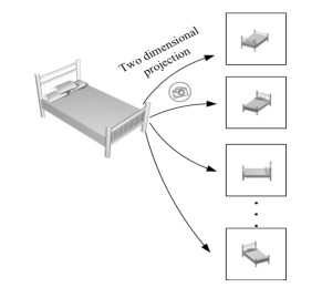
With the development of multimedia technology, the number of 3D models on the web or in databases is becoming increasingly larger and larger. It becomes more and more important to classify and retrieve 3D models. 3D model classification plays important roles in the mechanical design field, education field, medicine field and so on. Due to the 3D model's complexity and irregularity, it is difficult to classify 3D model correctly. Many methods of 3D model classification pay attention to local features from 2D views and neglect the 3D model's contour information, which cannot express it better. So, accuracy the of 3D model classification is poor. In order to improve the accuracy of 3D model classification, this paper proposes a method based on EfficientNet and Convolutional Neural Network (CNN) to classify 3D models, in which view feature and shape feature are used. The 3D model is projected into 2D views from different angles. EfficientNet is used to extract view feature from 2D views. Shape descriptors D1, D2, D3, Zernike moment and Fourier descriptors of 2D views are adopted to describe the 3D model and CNN is applied to extract shape feature. The view feature and shape feature are combined as discriminative features. Then, the softmax function is used to determine the 3D model's category. Experiments are conducted on ModelNet 10 dataset. Experimental results show that the proposed method achieves better than other methods.

| [1] |
J. W. Tangelder, R. C. Veltkamp, A survey of content based 3D shape retrieval methods, Multimedia Tools Appl., 39 (2008), 441–471. https://doi.org/10.1007/s11042-007-0181-0 doi: 10.1007/s11042-007-0181-0

|
| [2] |
H. Y. Zhou, A. A. Liu, W. Z. Nie, J. Nie, Multi-view saliency guided deep neural network for 3-D object retrieval and classification, IEEE Trans. Multimedia, 22 (2020), 1496–1506. https://doi.org/10.1109/TMM.2019.2943740 doi: 10.1109/TMM.2019.2943740
|
| [3] | C. R. Qi, H. Su, M. Nießner, A. Dai, M. Yan, L. Guibas, Volumetric and multi-view CNNs for object classification on 3D data, in 2016 IEEE Conference on Computer Vision and Pattern Recognition (CVPR), (2016), 5648–5656. https://doi.org/10.1109/CVPR.2016.609 |
| [4] |
X. A. Li, L. Y. Wang, J. Lu, Multiscale receptive fields graph attention network for point cloud classification, Complexity, 2021 (2021), 1076–2787. https://doi.org/10.1155/2021/8832081 doi: 10.1155/2021/8832081
|
| [5] | Y. L. Zhang, J. T. Sun, M. K. Chen, Q. Wang, Y. Yuan, R. Ma, Multi-weather classification using evolutionary algorithm on EfficientNet, in 2021 IEEE International Conference on Pervasive Computing and Communications Workshops and other Affiliated Events, (2021), 546–551. https://doi.org/10.1109/PerComWorkshops51409.2021.9430939 |
| [6] |
W. Nie, K. Wang, Q. Liang, R. He, Panorama based on multi-channel-attention CNN for 3D model recognition, Multimedia Syst., 25 (2019), 655–662. https://doi.org/10.1007/s00530-018-0600-2 doi: 10.1007/s00530-018-0600-2
|
| [7] |
A. A. Liu, F. B. Guo, H. Y. Zhou, W. Li, D. Song, Semantic and context information fusion network for view-based 3D model classification and retrieval, IEEE Access, 8 (2020), 155939–155950. https://doi.org/10.1109/ACCESS.2020.3018875 doi: 10.1109/ACCESS.2020.3018875
|
| [8] |
F. Chen, R. Ji, L. Cao, Multimodal learning for view-based 3D object classification, Neurocomputing, 195 (2016), 23–29. https://doi.org/10.1016/j.neucom.2015.09.120 doi: 10.1016/j.neucom.2015.09.120
|
| [9] |
Q. Huang, Y. Wang, Z. Yin, View-based weight network for 3D object recognition, Image Vision Comput., 93 (2020). https://doi.org/10.1016/j.imavis.2019.11.006 doi: 10.1016/j.imavis.2019.11.006
|
| [10] |
Z. Zhang, H. Lin, X. Zhao, R. Ji, Y. Gao, Inductive multi-hypergraph learning and its application on view-based 3D object classification, IEEE Trans. Image Process., 27 (2018), 5957–5968. https://doi.org/10.1109/TIP.2018.2862625 doi: 10.1109/TIP.2018.2862625
|
| [11] |
K. Sfikas, I. Pratikakis, T. Theoharis, Ensemble of panorama-based convolutional neural networks for 3D model classification and retrieval, Comput. Graphics, 71 (2018), 208–218. https://doi.org/10.1016/j.cag.2017.12.001 doi: 10.1016/j.cag.2017.12.001
|
| [12] |
P. Ma, J. Ma, X. Wang, L. Yang, N. Wang, Deformable convolutional networks for multi-view 3D shape classification, Electron. Lett., 54 (2018), 1373–1375. https://doi.org/10.1049/el.2018.6851 doi: 10.1049/el.2018.6851
|
| [13] |
M. F. Alotaibi, M. Omri, S. Abdel-Khalek, E. Khalil, R. Mansour, Computational intelligence-based harmony search algorithm for real-time object detection and tracking in video surveillance systems, Mathematics, 10 (2022), 1–16. https://doi.org/10.3390/math10050733 doi: 10.3390/math10050733
|
| [14] |
Q. Lin, Z. Wang, Y. Y. Chen, P. Zhong, Supervised multi-view classification via the sparse learning joint the weighted elastic loss, Signal Process., 191 (2022). https://doi.org/10.1016/j.sigpro.2021.108362 doi: 10.1016/j.sigpro.2021.108362
|
| [15] |
J. Yang, S. Wang, P. Zhou, Recognition and classification for three-dimensional model based on deep voxel convolution neural network, Acta Optica Sinica, 39 (2019), 1–11. http://dx.doi.org/10.3788/AOS201939.0415007 doi: 10.3788/AOS201939.0415007
|
| [16] |
T. Wang, W. Tao, C. M. Own, X. Lou, Y. Zhao, The layerizing voxpoint annular convolutional network for 3D shape classification, Comput. Graphics Forum, 39 (2020), 291–300. https://doi.org/10.1111/cgf.14145 doi: 10.1111/cgf.14145
|
| [17] |
Z. Liu, S. Wei, Y. Tian, S. Ji, Y. Sung, L. Wen, VB-Net: voxel-based broad learning network for 3D object classification, Appl. Sci., 10 (2020). https://doi.org/10.3390/app10196735 doi: 10.3390/app10196735
|
| [18] |
C. Wang, M. Cheng, F. Sohel, M. Bennamoun, J. Li, NormalNet: a voxel-based CNN for 3D object classification and retrieval, Neurocomputing, 323 (2019), 139–147. https://doi.org/10.1016/j.neucom.2018.09.075 doi: 10.1016/j.neucom.2018.09.075
|
| [19] |
A. Muzahid, W. Wan, F. Sohel, N. Ullah Khan, O. Villagómez, H. Ullah, 3D object classification using a volumetric deep neural network: an efficient octree guided auxiliary learning approach, IEEE Access, 8 (2020), 23802–23816. https://doi.org/10.1109/ACCESS.2020.2968506 doi: 10.1109/ACCESS.2020.2968506
|
| [20] |
Z. Kang, J. Yang, R. Zhong, Y. Wu, Z. Shi, R. Lindenbergh, Voxel-based extraction and classification of 3D pole-like objects from mobile LiDAR point cloud data, IEEE J. Sel. Top. Appl. Earth Obs. Remote Sens., 11 (2018), 4287–4298. https://doi.org/10.1109/JSTARS.2018.2869801 doi: 10.1109/JSTARS.2018.2869801
|
| [21] |
P. S. Wang, Y. Liu, Y. X. Guo, C. Sun, X. Tong, O-CNN: octree-based convolutional neural networks for 3D shape analysis, ACM Trans. Graph, 36 (2017), 1–11. https://doi.org/10.1145/3072959.3073608 doi: 10.1145/3072959.3073608
|
| [22] |
R. Guo, Y. Zhou, J. Zhao, Y. Man, M. Liu, R. Yao, et al., Point cloud classification by dynamic graph CNN with adaptive feature fusion, IET Comput. Vision, 15 (2021), 235–244. https://doi.org/10.1049/cvi2.12039 doi: 10.1049/cvi2.12039
|
| [23] |
X. Y. Gao, Y. Z. Wang, C. X. Zhang, J. Lu, Multi-head self-attention for 3D point cloud classification, IEEE Access, 9 (2021), 18137–18147. https://doi.org/10.1109/ACCESS.2021.3050488 doi: 10.1109/ACCESS.2021.3050488
|
| [24] |
C. Ma, Y. Guo, J. Yang, W. An, Learning multi-view representation with LSTM for 3-D shape recognition and retrieval, IEEE Trans. Multimedia, 21 (2019), 1169–1182. https://doi.org/10.1109/TMM.2018.2875512 doi: 10.1109/TMM.2018.2875512
|
| [25] |
A. Maligo, S. Lacroix, Classification of outdoor 3D lidar data based on unsupervised gaussian mixture models, IEEE Trans. Autom. Sci. Eng., 14 (2017), 5–16. https://doi.org/10.1109/TASE.2016.2614923 doi: 10.1109/TASE.2016.2614923
|
| [26] | Y. Zhang, M. Rabbat, A graph-CNN for 3D point cloud classification, in 2018 IEEE International Conference on Acoustics, Speech and Signal Processing, (2018), 6279–6283. https://doi.org/10.1109/ICASSP.2018.8462291 |
| [27] |
Y. T. Ng, C. M. Huang, Q. T. Li, J. Tian, RadialNet: a point cloud classification approach using local structure representation with radial basis function, Signal, Image Video Process., 14 (2020), 747–752. https://doi.org/10.1007/s11760-019-01607-0 doi: 10.1007/s11760-019-01607-0
|
| [28] |
Y. Wang, Y. Sun, Z. Liu, S. Sarma, M. Bronstein, J. Solomon, Dynamic graph CNN for learning on point clouds, ACM Trans. Graphics, 38 (2019), 1–12. https://doi.org/10.1145/3326362 doi: 10.1145/3326362
|
| [29] | D. Zhang, Z. Liu, X. Shi, Transfer learning on EfficientNet for remote sensing image classification, in 2020 5th International Conference on Mechanical, Control and Computer Engineering (ICMCCE), (2020), 2255–2258. https://doi.org/10.1109/ICMCCE51767.2020.00489 |
| [30] |
H. Alhichri, A. S. Alswayed, Y. Bazi, N. Ammour, N. Alajlan, Classification of remote sensing images using EfficientNet-B3 CNN model with attention, IEEE Access, 9 (2021), 14078–14094. https://doi.org/10.1109/ACCESS.2021.3051085 doi: 10.1109/ACCESS.2021.3051085
|
| [31] | M. Tan, Q. Le, Efficientnet: rethinking model scaling for convolutional neural networks, arXiv preprint, (2019), arXiv: 1905.11946. https://doi.org/10.48550/arXiv.1905.11946 |
| [32] | R. Kamble, P. Samanta, N. Singhal, Optic disc, cup and fovea detection from retinal images using U-Net++ with EfficientNet encoder, in Lecture Notes in Computer Science, (2020), 93–103. https://doi.org/10.1007/978-3-030-63419-3_10 |


Figures(5) / Tables(5)

Xue-Yao Gao, Bo-Yu Yang, Chun-Xiang Zhang. Combine EfficientNet and CNN for 3D model classification[J]. Mathematical Biosciences and Engineering, 2023, 20(5): 9062-9079. doi: 10.3934/mbe.2023398


 DownLoad: