Global dynamics of multiple delays within-host model for a hepatitis B virus infection of hepatocytes with immune response and drug therapy

Pensiri Yosyingyong; Ratchada Viriyapong; Pensiri Yosyingyong; Ratchada Viriyapong

doi:10.3934/mbe.2023319

Mathematical Biosciences and Engineering

2023, Volume 20, Issue 4: 7349-7386. doi: 10.3934/mbe.2023319

Previous Article Next Article

Research article

Global dynamics of multiple delays within-host model for a hepatitis B virus infection of hepatocytes with immune response and drug therapy

Pensiri Yosyingyong ,
Ratchada Viriyapong ^,

Department of Mathematics, Faculty of Science, Naresuan University, Phitsanulok, 65000, Thailand

Received: 01 November 2022 Revised: 08 February 2023 Accepted: 09 February 2023 Published: 14 February 2023

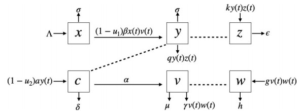
In this paper, a mathematical model describing the hepatitis B virus (HBV) infection of hepatocytes with the intracellular HBV-DNA containing capsids, cytotoxic T-lymphocyte (CTL), antibodies including drug therapy (blocking new infection and inhibiting viral production) with two-time delays is studied. It incorporates the delay in the productively infected hepatocytes and the delay in an antigenic stimulation generating CTL. We verify the positivity and boundedness of solutions and determine the basic reproduction number. The local and global stability of three equilibrium points (infection-free, immune-free, and immune-activated) are investigated. Finally, the numerical simulations are established to show the role of these therapies in reducing viral replication and HBV infection. Our results show that the treatment by blocking new infection gives more significant results than the treatment by inhibiting viral production for infected hepatocytes. Further, both delays affect the number of infections and duration i.e. the longer the delay, the more severe the HBV infection.

Keywords:

Citation: Pensiri Yosyingyong, Ratchada Viriyapong. Global dynamics of multiple delays within-host model for a hepatitis B virus infection of hepatocytes with immune response and drug therapy[J]. Mathematical Biosciences and Engineering, 2023, 20(4): 7349-7386. doi: 10.3934/mbe.2023319

Related Papers:

[1]	Jay Chu, Xiaozhe Hu, Lin Mu . A pressure-robust divergence free finite element basis for the Stokes equations. Electronic Research Archive, 2024, 32(10): 5633-5648. doi: 10.3934/era.2024261
[2]	Bin Wang, Lin Mu . Viscosity robust weak Galerkin finite element methods for Stokes problems. Electronic Research Archive, 2021, 29(1): 1881-1895. doi: 10.3934/era.2020096
[3]	Kun Wang, Lin Mu . Numerical investigation of a new cut finite element method for Stokes interface equations. Electronic Research Archive, 2025, 33(4): 2503-2524. doi: 10.3934/era.2025111
[4]	Xiu Ye, Shangyou Zhang . A stabilizer free WG method for the Stokes equations with order two superconvergence on polytopal mesh. Electronic Research Archive, 2021, 29(6): 3609-3627. doi: 10.3934/era.2021053
[5]	Chunmei Wang . Simplified weak Galerkin finite element methods for biharmonic equations on non-convex polytopal meshes. Electronic Research Archive, 2025, 33(3): 1523-1540. doi: 10.3934/era.2025072
[6]	Jun Pan, Yuelong Tang . Two-grid $ H^1 $-Galerkin mixed finite elements combined with $ L1 $ scheme for nonlinear time fractional parabolic equations. Electronic Research Archive, 2023, 31(12): 7207-7223. doi: 10.3934/era.2023365
[7]	Derrick Jones, Xu Zhang . A conforming-nonconforming mixed immersed finite element method for unsteady Stokes equations with moving interfaces. Electronic Research Archive, 2021, 29(5): 3171-3191. doi: 10.3934/era.2021032
[8]	Hongze Zhu, Chenguang Zhou, Nana Sun . A weak Galerkin method for nonlinear stochastic parabolic partial differential equations with additive noise. Electronic Research Archive, 2022, 30(6): 2321-2334. doi: 10.3934/era.2022118
[9]	Jiwei Jia, Young-Ju Lee, Yue Feng, Zichan Wang, Zhongshu Zhao . Hybridized weak Galerkin finite element methods for Brinkman equations. Electronic Research Archive, 2021, 29(3): 2489-2516. doi: 10.3934/era.2020126
[10]	Nisachon Kumankat, Kanognudge Wuttanachamsri . Well-posedness of generalized Stokes-Brinkman equations modeling moving solid phases. Electronic Research Archive, 2023, 31(3): 1641-1661. doi: 10.3934/era.2023085

Abstract

1. Introduction

In this manuscript, we detail the development of a new stabilizer-free weak Galerkin (WG) finite element method of any polynomial order in 2D and 3D, on triangular and tetrahedral meshes respectively, for obtaining the solutions of the stationary Stokes equations: Find unknown functions ${\bf{u}}$ (velocity) and $p$ (pressure) such that

$\begin{align} -\mu \Delta {\bf{u}}+\nabla p& = {{\bf{f}}}\quad \mbox{in}\;\Omega, \end{align}$

(1.1)

$\begin{align} \nabla\cdot {\bf{u}} & = 0\quad \mbox{in}\;\Omega, \end{align}$

(1.2)

$\begin{align} {\bf{u}}& = 0\quad \mbox{on}\; \partial\Omega, \end{align}$

(1.3)

where the viscosity $\mu > 0$ , and the domain $\Omega$ is a polygon or a polyhedron in $\mathbb{R}^d\; (d = 2, 3)$ .

The new pressure-robust, stabilizer-free WG method has a new variational formulation. Find ${\bf{u}}_h\in V_h$ and $p_h\in W_h$ such that

$\begin{align} (\mu \nabla_w {\bf{u}}_h, \nabla_w {\bf{v}})+(\nabla_w p_h, {\bf{v}})& = ({\bf{f}}, {\bf{v}}) \quad\forall {\bf{v}}\in V_h, \end{align}$

(1.4)

$\begin{align} ( {\bf{u}}_h, \nabla_wq)& = 0\qquad \forall q\in W_h, \end{align}$

(1.5)

where $\nabla_w$ denotes weak gradients to be defined in (2.3) and (2.4), and $V_h$ and $W_h$ are $P_k$ and $P_{k-1}$ WG finite element spaces, to be defined in (2.1) and (2.2), respectively. Some studies on the WG methods are as follows: the parabolic equation ^[1,2,3], with two-order superconvergence on triangular meshes ^[4], the convection-diffusion equation ^[5,6], 4th order problems ^[7,8], with the conforming discontinuous Galerkin formulation ^[9,10,11], the Navier-Stokes equations ^[12,13,14], with the discrete maximum principle ^[15], the second order elliptic equations ^[16,17], with the energy conservation ^[18], the Darcy flow ^[19,20], the Oseen equations ^[21], the Stokes equations with pressure-robustness ^[22,23,24], the Maxwell equations ^[25], the Cahn-Hilliard equation ^[26], the div-curl equations ^[27], with adaptive refinements ^[28,29], the biharmonic equation ^[30,31], the biharmonic equation with continuous finite elements^[32,33], the Stokes equations with $H({\operatorname{{div}}})$ elements ^[34,35], with two-order superconvergence under the CDG formulation ^[36,37], and with two-order superconvergence for the Stokes equations ^[38].

We note that the moment equation (1.1) is not tested by applying $H({\operatorname{{div}}}, \Omega)$ functions in (1.4), different from most other pressure-robust methods such as those detailed in ^[22,23,24], but is tested by using discontinuous polynomials. The pointwise divergence-free property (pressure-robustness) is achieved by introducing pressure face variables, i.e., $p_h = \{p_0, p_b\}$ where $p_b|_e\in P_k(e)$ on every face edge/triangle $e$ of a mesh $\mathcal T_h$ (see (2.2) below). The method was previously applied before in hybridized discontinuous Galerkin methods in ^[39].

It is shown that the WG finite element pair, $V_h-W_h$ , is inf-sup stable. The method is shown pressure robust, i.e., both errors of the velocity and the pressure are independent of the pressure $p$ and the viscosity $\mu$ in (1.1). This is necessary when $\mu$ is small. However, very few methods can achieve this. Under the inf-sup stability, we shall prove quasi-optimal approximation for the velocity in an $H^1$ -norm and in the $L^2$ norm. The quasi-optimal convergence for pressure in the $L^2$ norm is also proved. The theory is numerically verified by applying varying degrees of WG finite elements to both triangular and tetrahedral meshes.

2. The WG finite element method

Let ${ \mathcal T}_h$ be a mesh on the domain $\Omega$ , consisting of conforming shape-regular triangles or shape-regular tetrahedrons. Here we let $h_T$ be the element diameter of $T\in {{\mathcal T}}_h$ , and we let mesh size $h = \max_{T\in{{\mathcal T}}_h} h_T$ .

For $k\ge 1$ and given ${{\mathcal T}}_h$ , the finite element space for velocity is defined by

$\begin{align} \begin{aligned} V_h = \big\{ {\bf{v}} = \{ {\bf{v}}_0, {\bf{v}}_b\} & :\ {\bf{v}}_0|_{T}\in [P_{k}(T)]^d, \ T\in{{\mathcal T}}_h; \\ &\quad {\bf{v}}_b|_e\in [P_{k+1}(e)]^d, \ e\in \mathcal E_h; \ {\bf{v}}_b|_e = {{\mathbf 0}}, \ e \in \mathcal E_h\cap \partial \Omega \big\}, \end{aligned} \end{align}$

(2.1)

and the finite element space for pressure is defined by

$\begin{align} \begin{aligned} W_h = \{ q_h = \{q_0, q_b\} : & \ q_0|_T\in P_{k-1}(T), \ T\in \mathcal{T}; \ q_b|_e\in P_k(e), \\ & \ e\in \mathcal E_h; (q_0, 1)_{\mathcal T_h}+\langle q_b, 1\rangle_{\partial \mathcal T_h} = 0 \}, \end{aligned} \end{align}$

(2.2)

where $P_k(e)$ and $P_k(T)$ denote the space of polynomials of degree $k$ or less on the edge/triangle $e$ and triangle/tetrahedron $T$ respectively, $(\cdot, \cdot)_{\mathcal T_h} = \sum_{T\in \mathcal T_h} (\cdot, \cdot)_T$ and $\langle\cdot, \cdot \rangle_{\partial \mathcal T_h} = \sum_{T\in \mathcal T_h} \langle \cdot, \cdot\rangle_{\partial T}$ .

For a function ${\bf{v}}\in V_h$ , the $(k+1)$ -degree weak gradient $\nabla_w {\bf{v}}$ is a piecewise polynomial on the mesh $\mathcal T_h$ , $\nabla_w {\bf{v}}|_T \in [P_{k+1}(T)]^{d\times d}$ , such that

$\begin{equation} \label{wg} (\nabla_w {\bf{v}}, \ \tau)_T = -( {\bf{v}}_0, \ \nabla\cdot \tau)_T+ {{\langle}} {\bf{v}}_b, \ \tau\cdot{{\bf{n}}} {{\rangle}}_{{\partial T}}\quad\forall\tau\in [P_{k+1}(T)]^{d\times d}. \end{equation}$

(2.3)

For a function $q = \{q_0, q_b\}\in W_h$ , its weak gradient $\nabla_w q$ is defined as a piecewise vector-valued polynomial such that for each $T\in{{\mathcal T}}_h$ , $\nabla_w q \in [P_k(T)]^d$ satisfies

$\begin{equation} (\nabla_w q, {{\boldsymbol{\varphi}}})_T = -(q_0, \nabla\cdot{{\boldsymbol{\varphi}}})_T + \langle q_b, {{\boldsymbol{\varphi}}}\cdot{{\bf{n}}}\rangle_{\partial T}\quad \forall {{\boldsymbol{\varphi}}}\in [P_k(T)]^d. \end{equation}$

(2.4)

We denote by $\Pi_k$ the local/element-wise $L^2$ -orthogonal projection onto $[P_k(T)]^j$ where $j = 1, \; d, \; d \; \times\; d$ and $T\in{{\mathcal T}}_h$ . Let $\Pi_k^b$ be a generic edge/face-wise defined $L^2$ projection onto $[P_k(e)]^j$ for $e\in{{\partial T}}$ . Define ${\bf{Q}}_h {\bf{u}} = \{\Pi_k {\bf{u}}, \Pi_{k+1}^b {\bf{u}}\}\in V_h$ and $Q_h p = \{\Pi_{k-1}p, \Pi_k^bp\}\in W_h$ .

Lemma 2.1. Let $\boldsymbol\phi\in [H_0^1(\Omega)]^d$ and $\psi\in H^1(\Omega)$ , then, for $T\in{{\mathcal T}}_h$

$\begin{eqnarray} \nabla_w {\bf{Q}}_h\boldsymbol\phi & = &\Pi_{k+1}\nabla\boldsymbol\phi, \end{eqnarray}$

(2.5)

$\begin{eqnarray} \nabla_w Q_h\psi & = &\Pi_{k}\nabla\psi. \end{eqnarray}$

(2.6)

Proof. Using (2.3) and integration by parts, we obtain the following for any $\tau\in [P_{k+1}(T)]^{d\times d}$ :

$\begin{eqnarray*} (\nabla_w Q_h\boldsymbol\phi, \tau)_T & = & -(\Pi_k\boldsymbol\phi, \nabla\cdot\tau)_T +\langle \Pi_{k+1}^b\boldsymbol\phi, \tau\cdot{{\bf{n}}}\rangle_{{{\partial T}}}\\ & = & -(\boldsymbol\phi, \nabla\cdot\tau)_T +\langle \boldsymbol\phi, \tau\cdot{{\bf{n}}}\rangle_{{{\partial T}}}\\ & = &(\nabla \boldsymbol\phi, \tau)_T = (\Pi_{k+1}\nabla\boldsymbol\phi, \tau)_T. \end{eqnarray*}$

This implies that (2.5) holds. The scalar version, (2.6), is proved in the same manner.

For any function $\varphi\in H^1(T)$ , the following trace inequality holds true:

$\begin{equation} \|\varphi\|_{e}^2 \leq C \left( h_T^{-1} \|\varphi\|_T^2 + h_T \|\nabla \varphi\|_{T}^2\right). \end{equation}$

(2.7)

We define two semi-norms $||| {\bf{v}}|||$ and $\| {\bf{v}}\|_{1, h}$ for any ${\bf{v}}\in V_h$ :

$\begin{eqnarray} ||| {\bf{v}}|||^2 & = & (\nabla_w {\bf{v}}, \nabla_w {\bf{v}}), \end{eqnarray}$

(2.8)

$\begin{eqnarray} \| {\bf{v}}\|_{1, h}^2& = &\sum\limits_{T\in {{\mathcal T}}_h}\|\nabla {\bf{v}}_0\|_T^2+\sum\limits_{T\in{{\mathcal T}}_h}h_T^{-1}\| {\bf{v}}_0- {\bf{v}}_b\|_{{{\partial T}}}^2. \end{eqnarray}$

(2.9)

We also define two semi-norms $||| q|||$ and $\|q\|_{1, h}$ for any $q\in W_h$ :

$\begin{eqnarray} ||| q|||^2 & = & (\nabla_w q, \nabla_w q), \end{eqnarray}$

(2.10)

$\begin{eqnarray} \|q\|_{1, h}^2& = &\sum\limits_{T\in {{\mathcal T}}_h}\|\nabla q_0\|_T^2+\sum\limits_{T\in{{\mathcal T}}_h}h_T^{-1}\|q_0-q_b\|_{{{\partial T}}}^2. \end{eqnarray}$

(2.11)

In fact, $\| {\bf{v}}\|_{1, h}$ is a norm in $V_h$ and $||| \cdot |||$ is also a norm in $V_h$ , as they have been proved in ^[4] by applying the norm equivalence as follows:

$\begin{equation} C_1\| {\bf{v}}\|_{1, h}\le ||| {\bf{v}}|||\le C_2 \| {\bf{v}}\|_{1, h} \quad\forall {\bf{v}}\in V_h, \end{equation}$

(2.12)

and

$\begin{equation} C_1\|q\|_{1, h}\le ||| q|||\le C_2 \|q\|_{1, h} \quad\forall q\in W_h. \end{equation}$

(2.13)

Lemma 2.2. The following inf-sup conditions hold, for all $q = \{q_0, q_b\}\in W_h$ and ${\bf{v}} = \{ {\bf{v}}_0, {\bf{v}}_b\}\in V_h$ :

$\begin{equation} \sup\limits_{ {\bf{v}}\in V_h}\frac{( {\bf{v}}_0, \nabla_wq)}{|||{\bf{v}}|||}\ge \beta \|q_0\|, \end{equation}$

(2.14)

and

$\begin{equation} \sup\limits_{ {\bf{v}}\in V_h}\frac{( {\bf{v}}_0, \nabla_wq)}{|||{\bf{v}}|||}\ge \beta h||| q|||, \end{equation}$

(2.15)

where $\beta > 0$ is independent of $h$ and $\mathcal T_h$ .

Proof. For any given $q = \{q_0, q_b\}\in W_h$ , it is known that there exists a function $\tilde {\bf{v}}\in H_0({\operatorname{{div}}}, \Omega)$ and $\tilde {\bf{v}}|_T\in [P_k(T)]^d$ (see, e.g., [40, (7.4)–(7.6)]) such that

$\begin{equation} \frac{(\nabla\cdot\tilde {\bf{v}}, q_0)}{|\tilde {\bf{v}}|_{1, h}}\ge C\|q_0\|, \end{equation}$

(2.16)

where

$|\tilde {\bf{v}}|_{1, h}^2 = \sum\limits_{T\in{{\mathcal T}}_h}(\|\nabla \tilde {\bf{v}}\|_T^2+h_T^{-1}\|[\tilde {\bf{v}}]\|_{{\partial T}}^2).$

Let

$\begin{align*} {\bf{v}} = \{\tilde {\bf{v}}, \tilde {\bf{v}}_b \}\in V_h, \quad{\operatorname{{ where }}} \ \tilde {\bf{v}}_b|_e = \begin{cases} \frac 12(\tilde {\bf{v}}|_{T_1} + \tilde {\bf{v}}|_{T_2}) & {\operatorname{{ if }}}\ e\in \mathcal E_h^0, \\ {{\mathbf 0}} & {\operatorname{{ if }}}\ e\in \mathcal E_h\cap \partial\Omega, \end{cases} \end{align*}$

where $T_1$ and $T_2$ are the two elements on the two sides of edge/triangle $e$ . For such specially defined ${\bf{v}}$ , we have

$\begin{align} \begin{aligned} \| {\bf{v}}\|_{1, h}^2& = \sum\limits_{T\in {{\mathcal T}}_h}(\|\nabla \tilde {\bf{v}}\|_T^2+h_T^{-1}\|\tilde {\bf{v}}-\{\tilde {\bf{v}}\}\|_{{{\partial T}}}^2) \\ & = \sum\limits_{T\in {{\mathcal T}}_h}(\|\nabla \tilde {\bf{v}}\|_T^2+h_T^{-1}\|[\tilde {\bf{v}}]\|_{{{\partial T}}}^2) = |\tilde {\bf{v}}|_{1, h}^2. \end{aligned} \end{align}$

(2.17)

It follows from (2.13) and (2.17) that

$\begin{equation} ||| {\bf{v}}|||\le C |\tilde {\bf{v}}|_{1, h}. \end{equation}$

(2.18)

By (2.4), we have

$\begin{eqnarray} (\tilde {\bf{v}}, \nabla_w q) = \sum\limits_{T\in{{\mathcal T}}_h} \left({{\langle}}\tilde {\bf{v}}\cdot{{\bf{n}}}, q_b {{\rangle}}_{{{\partial T}}}- (\nabla\cdot\tilde {\bf{v}}, q_0)_T\right) = -(\nabla\cdot\tilde {\bf{v}}, q_0) . \end{eqnarray}$

(2.19)

Combining (2.16), (2.19) and (2.18) implies that

$\begin{eqnarray*} \frac{|(\tilde {\bf{v}}, \nabla_w q)|}{|||{\bf{v}}|||}& = &\frac{|(\nabla\cdot\tilde {\bf{v}}, q_0)|}{|||{\bf{v}}|||} \ge\frac{|(\nabla\cdot\tilde {\bf{v}}, q_0)|}{\|\tilde {\bf{v}}\|_{1, h}}\ge \beta\|q_0\|, \end{eqnarray*}$

which implies (2.14).

Next we shall derive (2.15). For any ${\bf{v}} = \{ {\bf{v}}_0, {{\mathbf 0}}\}\in V_h$ and $\tau\in [P_{k+1}(T)]^{d\times d}$ , we have the following by (2.3), (2.7) and the inverse inequalities:

$\begin{align*} (\nabla_w {\bf{v}}, \tau)_{T}& = -( {\bf{v}}_0, \nabla\cdot\tau)_{T} = (\nabla {\bf{v}}_0, \tau)_{T}-{{\langle}} {\bf{v}}_0, \tau\cdot{{\bf{n}}}{{\rangle}}_{{{\partial T}}} \\ &\le \|\nabla {\bf{v}}_0\|_T\|\tau\|_T+Ch_T^{-1/2}\| {\bf{v}}_0\|_{{\partial T}}\|\tau\|_T, \end{align*}$

which implies that

$\begin{eqnarray} |||{\bf{v}}|||\le Ch^{-1}\| {\bf{v}}_0\|. \end{eqnarray}$

(2.20)

It follows from (2.20) that for any ${\bf{v}} = \{ {\bf{v}}_0, {{\mathbf 0}}\}\in V_h$

$\begin{align*} \frac{|( {\bf{v}}_0, \nabla_w q)|}{|||{\bf{v}}|||} &\ge Ch\frac{|( {\bf{v}}_0, \nabla_w q)|}{\| {\bf{v}}_0\|}. \end{align*}$

Then we have

$\begin{align*} \sup\limits_{ {\bf{v}}\in V_h}\frac{|( {\bf{v}}_0, \nabla_w q)|}{|||{\bf{v}}|||} &\ge Ch\sup\limits_{ {\bf{v}}\in V_h}\frac{|( {\bf{v}}_0, \nabla_w q)|}{\| {\bf{v}}_0\|}\ge \beta h\|\nabla_wq\|, \end{align*}$

which implies (2.15). This completes the proof of the lemma.

Lemma 2.3. There is a unique solution for the WG finite element equations (1.4) and (1.5).

Proof. We only need to show that zero is the unique solution of (1.4) and (1.5) if ${{\bf{f}}} = {{\mathbf 0}}$ . We let ${{\bf{f}}} = {{\mathbf 0}}$ and ${\bf{v}} = {\bf{u}}_h$ in (1.4) and $q = p_h$ in (1.5). By summing the two equations, we get

$(\nabla_w {\bf{u}}_h, \ \nabla_w {\bf{u}}_h) = 0.$

It implies that $\nabla_w {\bf{u}}_h = 0$ on $T$ . By (2.12), we also obtain that $\| {\bf{u}}_h\|_{1, h} = 0$ . Thus, ${\bf{u}}_h = {{\mathbf 0}}$ .

Since ${\bf{u}}_h = {{\mathbf 0}}$ and ${{\bf{f}}} = {{\mathbf 0}}$ , (1.4) is reduced to $({\bf{v}}_0, \nabla_wp_h) = 0$ for any ${\bf{v}} = \{ {\bf{v}}_0, {\bf{v}}_b\}\in V_h$ . Then the inf-sup conditions (2.15) and (2.14) imply that $\nabla_wp_h = 0$ and $p_0 = 0$ . By (2.13), we have that $\|p_h\|_{1, h} = 0$ and $p_0 = p_b = 0$ on ${{\partial T}}$ . We have proved the lemma.

3. Error equations

To derive the equations that the errors satisfy, we introduce ${\bf{e}}_h = {\bf{Q}}_h {\bf{u}}- {\bf{u}}_h$ and $\epsilon_h = Q_hp-p_h$ .

Lemma 3.1. [, Theorem 3.1] For $\tau\in [H^{k+2}(\Omega)]^d$ , a quasi-projection $\Pi_h$ can be defined such that $\Pi_h\tau\in [H({\operatorname{{div}}}, \Omega)]^d$ , $\Pi_h\tau|_T\in [P_{k+1}(T)]^{d\times d}$ and for ${\bf{v}}_0\in [P_k(T)]^d$ ,

$\begin{eqnarray} (\nabla\cdot\tau, \; {\bf{v}}_0)_T& = &(\nabla\cdot\Pi_h\tau, \; {\bf{v}}_0)_T, \end{eqnarray}$

(3.1)

$\begin{eqnarray} -(\nabla\cdot\tau, \; {\bf{v}}_0)& = &(\Pi_h\tau, \;\nabla_w {\bf{v}}), \end{eqnarray}$

(3.2)

$\begin{eqnarray} \|\Pi_h\tau-\tau\|&\le& Ch^{k+2}|\tau|_{k+2}, \end{eqnarray}$

(3.3)

where $|\cdot|_{k+2}$ is the semi- $H^{k+2}$ Sobolev norm on the space.

Lemma 3.2. [, Theorem 3.1] Let $\tau\in H^{k+1}(\Omega)$ . A quasi-projection $\pi_h$ can be defined such that $\pi_h\tau\in H({\operatorname{{div}}}, \Omega)$ , $\pi_h\tau|_T\in [P_{k}(T)]^d$ and for $q_0\in P_{k-1}(T)$ ,

$\begin{eqnarray} (\nabla\cdot\tau, \;q_0)_T& = &(\nabla\cdot\pi_h\tau, \;q_0)_T, \end{eqnarray}$

(3.4)

$\begin{eqnarray} -(\nabla\cdot\tau, \;q_0)& = &(\pi_h\tau, \;\nabla_w q), \end{eqnarray}$

(3.5)

$\begin{eqnarray} \|\pi_h\tau-\tau\|&\le& Ch^{k+1}|\tau|_{k+1}, \end{eqnarray}$

(3.6)

where $|\cdot|_{k+1}$ is the semi- $H^{k+1}$ Sobolev norm on the space.

Lemma 3.3. For any ${\bf{v}}\in V_h$ and $q\in W_h$ , the following error equations hold true:

$\begin{eqnarray} (\mu \nabla_w {\bf{e}}_h, \; \nabla_w {\bf{v}})+(\nabla_w\epsilon_h, \; {\bf{v}}_0)& = &e_1( {\bf{u}}, {\bf{v}}), \end{eqnarray}$

(3.7)

$\begin{eqnarray} ( {\bf{e}}_0, \ \nabla_w q)& = &e_2( {\bf{u}}, q), \end{eqnarray}$

(3.8)

where

$\begin{eqnarray} e_1( {\bf{u}}, \ {\bf{v}})& = &\mu (\Pi_{k+1}\nabla {\bf{u}}-\Pi_h\nabla {\bf{u}}, \nabla_w {\bf{v}}), \end{eqnarray}$

(3.9)

$\begin{eqnarray} e_2( {\bf{u}}, q)& = &(\Pi_k {\bf{u}}-\pi_{h} {\bf{u}}, \nabla_w q). \end{eqnarray}$

(3.10)

Proof. First, we test (1.1) by applying ${\bf{v}}_0$ with ${\bf{v}} = \{ {\bf{v}}_0, {\bf{v}}_b\}\in V_h$ to obtain

$\begin{equation} -(\mu \Delta {\bf{u}}, \; {\bf{v}}_0)+(\nabla p, \ {\bf{v}}_0) = ({{\bf{f}}}, \; {\bf{v}}_0). \end{equation}$

(3.11)

It follows from (3.2) and (2.5) that

$\begin{equation} -(\mu \nabla\cdot\nabla {\bf{u}}, \; {\bf{v}}_0) = (\mu \Pi_h\nabla {\bf{u}}, \; \nabla_w {\bf{v}}) = (\mu \nabla_w {\bf{Q}}_h {\bf{u}}, \; \nabla_w {\bf{v}})-e_1( {\bf{u}}, {\bf{v}}). \end{equation}$

(3.12)

It follows from (2.6) that

$\begin{eqnarray} (\nabla p, \ {\bf{v}}_0)& = & (\Pi_k\nabla p, \ {\bf{v}}_0) = (\nabla_w Q_h p, \ {\bf{v}}_0). \end{eqnarray}$

(3.13)

We substitute (3.12) and (3.13) into (3.11) to obtain

$\begin{equation} (\mu \nabla_w {\bf{Q}}_h {\bf{u}}, \nabla_w {\bf{v}})+(\mu \nabla_w Q_h p, \ {\bf{v}}_0) = ({{\bf{f}}}, {\bf{v}}_0)+e_1( {\bf{u}}, {\bf{v}}). \end{equation}$

(3.14)

We subtract (3.14) from (1.4) to get

$\begin{equation} (\mu \nabla_w {\bf{e}}_h, \nabla_w {\bf{v}})+(\mu \nabla_w \epsilon_h, \ {\bf{v}}_0) = e_1( {\bf{u}}, {\bf{v}})\quad\forall {\bf{v}}\in V_h . \end{equation}$

(3.15)

Multiplying (1.2) by $q = \{q_0, q_b\}\in W_h$ , by applying (3.2), it follows that

$\begin{equation} 0 = (\nabla\cdot {\bf{u}}, \ q_0) = -(\pi_h {\bf{u}}, \nabla_w q) = -(\Pi_k {\bf{u}}, \nabla_w q)+e_2( {\bf{u}}, q), \end{equation}$

(3.16)

which implies that

$\begin{equation} (\Pi_k {\bf{u}}, \nabla_w q) = e_2( {\bf{u}}, q). \end{equation}$

(3.17)

The difference between (3.17) and (1.5) implies (3.8). We have proved the lemma.

4. Quasi-optimal finite element solutions

We shall first prove the optimal order error estimates of the $|||\cdot|||$ norm for the velocity ${\bf{u}}_h$ , and of the $L^2$ norm for the pressure $p_h$ .

Lemma 4.1. Let ${\bf{u}}\in [H^{k+1}(\Omega)]^d$ , ${\bf{v}}\in V_h$ and $q\in W_h$ . The following estimates hold:

$\begin{eqnarray} |e_1( {\bf{u}}, \ {\bf{v}})|&\le& C \mu h^{k}| {\bf{u}}|_{k+1}||| {\bf{v}}|||, \end{eqnarray}$

(4.1)

$\begin{eqnarray} |e_2( {\bf{u}}, \ q)|&\le& C h^{k+1}| {\bf{u}}|_{k+1}||| q|||, \end{eqnarray}$

(4.2)

where $e_1(\cdot, \cdot)$ and $e_2(\cdot, \cdot)$ have been defined in (3.9) and (3.10), respectively.

Proof. By the Cauchy-Schwarz inequality, the definitions of $\Pi_{k+1}$ and $\Pi_h$ , we compute

$\begin{eqnarray*} |e_1( {\bf{u}}, \ {\bf{v}})|& = &\mu |(\Pi_{k+1}\nabla {\bf{u}}-\Pi_h\nabla {\bf{u}}, \nabla_w {\bf{v}})|\\ &\le & C\mu h^{k}| {\bf{u}}|_{k+1}||| {\bf{v}}|||. \end{eqnarray*}$

Similarly, we have

$\begin{eqnarray*} |e_2( {\bf{u}}, \ q)|& = &|(\pi_{h} {\bf{u}}-\Pi_k {\bf{u}}, \nabla_w q)|\\ &\le & Ch^{k+1}| {\bf{u}}|_{k+1}\| ||| q|||. \end{eqnarray*}$

We have proved the lemma.

Theorem 4.1. Let $({\bf{u}}, p)\in \big([H^{k+1}(\Omega)]^d \cap [H^1_0(\Omega)]^d \big) \times \big(H^k(\Omega)\cap L^2_0(\Omega)\big)$ be the solutions of (1.1)–(1.3). Let $({\bf{u}}_h, p_h)\in V_h \times W_h$ be the solutions of (1.4) and (1.5). Then, the following error estimates hold true:

$\begin{eqnarray} ||| {\bf{Q}}_h {\bf{u}}- {\bf{u}}_h||| &\le& Ch^{k}| {\bf{u}}|_{k+1}, \end{eqnarray}$

(4.3)

$\begin{eqnarray} h||| Q_hp-p_h|||+\|\Pi_{k-1}p-p_0\|&\le& C \mu h^{k}| {\bf{u}}|_{k+1}. \end{eqnarray}$

(4.4)

Proof. It follows from (3.7) that for any ${\bf{v}} = \{ {\bf{v}}_0, {\bf{v}}_b\}\in V_h$ , by (4.1), we have

$\begin{eqnarray} |(\nabla_w\epsilon_h, \; {\bf{v}}_0)|& = &|(\mu \nabla_w {\bf{e}}_h, \; \nabla_w {\bf{v}})-e_1( {\bf{u}}, {\bf{v}})|\\ &\le& C \mu (||| {\bf{e}}_h||| +h^{k}| {\bf{u}}|_{k+1})|||{\bf{v}}|||. \end{eqnarray}$

(4.5)

Then applying the estimate (4.5) and (2.15) yields

$\begin{eqnarray} h|||\epsilon_h||| &\le& C \mu (||| {\bf{e}}_h||| +h^{k}| {\bf{u}}|_{k+1}). \end{eqnarray}$

(4.6)

By letting ${\bf{v}} = {\bf{e}}_h$ in (3.7) and $q = \epsilon_h$ in (3.8), and by using (3.8), we have

$\begin{align*} ||| {\bf{e}}_h|||^2& = |\mu^{-1} e_1( {\bf{u}}, {\bf{e}}_h)-e_2( {\bf{u}}, \epsilon_h)|. \end{align*}$

It then follows from (4.1), (4.2) and (4.6) that

$\begin{align*} ||| {\bf{e}}_h|||^2 &\le Ch^{k}| {\bf{u}}|_{k+1}||| {\bf{e}}_h|||+Ch^{k}| {\bf{u}}|_{k+1}h||| \epsilon_h||| \\ &\le Ch^{k}| {\bf{u}}|_{k+1}||| {\bf{e}}_h|||+Ch^{2k}| {\bf{u}}|_{k+1}^2, \end{align*}$

which implies (4.3). The estimate (4.4) follows from (4.5), (4.3) and the inf-sup conditions (2.14) and (2.15). We have proved the theorem.

We shall derive next the optimal-order convergence for velocity in the $L^2$ norm by using the duality argument. Recall that ${\bf{e}}_h = \{ {\bf{e}}_0, {\bf{e}}_b\} = {\bf{Q}}_h {\bf{u}}- {\bf{u}}_h$ and $\epsilon_h = Q_hp-p_h$ . Consider the problem of seeking $({{\boldsymbol{\psi}}}, \xi)$ such that

$\begin{eqnarray} -\mu \Delta{{\boldsymbol{\psi}}}+\nabla \xi& = {\bf{e}}_0 &\quad \mbox{in}\;\Omega, \end{eqnarray}$

(4.7)

$\begin{eqnarray} \nabla\cdot{{\boldsymbol{\psi}}}& = 0 &\quad\mbox{in}\;\Omega, \end{eqnarray}$

(4.8)

$\begin{eqnarray} {{\boldsymbol{\psi}}}& = 0 &\quad\mbox{on}\;\partial\Omega. \end{eqnarray}$

(4.9)

Assume that the duality problem given by (4.7)–(4.9) has the ${{\bf H}}^{2}(\Omega)\times H^1(\Omega)$ -regularity property that the solution $({{\boldsymbol{\psi}}}, \xi)\in {{\bf H}}^{2}(\Omega)\times H^1(\Omega)$ and the following a priori estimate holds true:

$\begin{eqnarray} \mu \|{{\boldsymbol{\psi}}}\|_{2}+\|\xi\|_1&\le& C\| {\bf{e}}_0\|. \end{eqnarray}$

(4.10)

We need the following lemma first.

Lemma 4.2. For any ${\bf{v}}\in V_h$ and $q\in W_h$ , the following equations hold true:

$\begin{eqnarray} (\mu \nabla_w {\bf{Q}}_h{{\boldsymbol{\psi}}}, \; \nabla_w {\bf{v}})+( \nabla_wQ_h\xi, \; {\bf{v}}_0) & = &( {\bf{e}}_0, {\bf{v}}_0)+e_3({{\boldsymbol{\psi}}}, {\bf{v}}), \end{eqnarray}$

(4.11)

$\begin{eqnarray} ( \Pi_k{{\boldsymbol{\psi}}}, \nabla_w q)& = &e_4({{\boldsymbol{\psi}}}, q) , \end{eqnarray}$

(4.12)

where ${{\boldsymbol{\psi}}}$ and $\xi$ are defined in (4.7), and

$\begin{eqnarray*} e_3({{\boldsymbol{\psi}}}, \ {\bf{v}})& = &\langle \mu (\nabla{{\boldsymbol{\psi}}}-\Pi_{k+1}\nabla{{\boldsymbol{\psi}}})\cdot{{\bf{n}}}, \; {\bf{v}}_0- {\bf{v}}_b\rangle_{\partial{{\mathcal T}}_h}, \\ e_4({{\boldsymbol{\psi}}}, \;q)& = &{{\langle}} ({{\boldsymbol{\psi}}}-\Pi_k{{\boldsymbol{\psi}}})\cdot{{\bf{n}}}, q_0-q_b{{\rangle}}_{\partial{{\mathcal T}}_h}. \end{eqnarray*}$

Proof. Testing (4.7) by applying ${\bf{v}}_0$ with ${\bf{v}} = \{ {\bf{v}}_0, {\bf{v}}_b\}\in V_h$ gives

$\begin{equation} -(\mu \Delta{{\boldsymbol{\psi}}}, \; {\bf{v}}_0)+(\nabla \xi, \ {\bf{v}}_0) = ( {\bf{e}}_0, \; {\bf{v}}_0). \end{equation}$

(4.13)

By performing integration by parts, and setting $\langle\nabla {{\boldsymbol{\psi}}}\cdot{{\bf{n}}}, {\bf{v}}_b\rangle_{\partial{{\mathcal T}}_h} = 0$ , we derive

$\begin{equation} -(\Delta{{\boldsymbol{\psi}}}, \; {\bf{v}}_0) = (\nabla{{\boldsymbol{\psi}}}, \nabla {\bf{v}}_0)_{{{\mathcal T}}_h}- \langle \nabla {{\boldsymbol{\psi}}}\cdot{{\bf{n}}}, {\bf{v}}_0- {\bf{v}}_b\rangle_{\partial{{\mathcal T}}_h}. \end{equation}$

(4.14)

By integration by parts, and given(2.3) and (2.5), we have

$\begin{eqnarray} (\nabla {{\boldsymbol{\psi}}}, \nabla {\bf{v}}_0)_{{{\mathcal T}}_h}& = &(\Pi_{k+1}\nabla{{\boldsymbol{\psi}}}, \nabla {\bf{v}}_0)_{{{\mathcal T}}_h}\\ & = &-( {\bf{v}}_0, \nabla\cdot (\Pi_{k+1}\nabla {{\boldsymbol{\psi}}}))_{{{\mathcal T}}_h}+\langle {\bf{v}}_0, \Pi_{k+1}\nabla {{\boldsymbol{\psi}}}\cdot{{\bf{n}}}\rangle_{\partial{{\mathcal T}}_h}\\ & = &(\Pi_{k+1}\nabla {{\boldsymbol{\psi}}}, \nabla_w {\bf{v}})_{{{\mathcal T}}_h}+\langle {\bf{v}}_0- {\bf{v}}_b, \Pi_{k+1}\nabla \psi\cdot{{\bf{n}}}\rangle_{\partial{{\mathcal T}}_h}\\ & = &( \nabla_w {\bf{Q}}_h{{\boldsymbol{\psi}}}, \nabla_w {\bf{v}})_{{{\mathcal T}}_h}+\langle {\bf{v}}_0- {\bf{v}}_b, \Pi_{k+1}\nabla {{\boldsymbol{\psi}}}\cdot{{\bf{n}}}\rangle_{\partial{{\mathcal T}}_h}. \end{eqnarray}$

(4.15)

Combining (4.14) and (4.15) gives

$\begin{eqnarray} -(\mu \Delta{{\boldsymbol{\psi}}}, \; {\bf{v}}_0)& = &( \mu \nabla_w {\bf{Q}}_h{{\boldsymbol{\psi}}}, \nabla_w v)-e_3({{\boldsymbol{\psi}}}, {\bf{v}}). \end{eqnarray}$

(4.16)

By applying the definition of $\Pi_k$ , (2.6), and (3.13), we obtain

$\begin{equation} (\nabla \xi, \ {\bf{v}}_0) = (\Pi_k\nabla \xi, \ {\bf{v}}_0) = (\nabla_w Q_h\xi, \ {\bf{v}}_0). \end{equation}$

(4.17)

Combining (4.16) and (4.17) with (4.13) yields (4.11).

Testing (4.8) by applying $q_0$ with $q = \{q_0, q_b\}\in W_h$ gives

$\begin{eqnarray} (\nabla\cdot{{\boldsymbol{\psi}}}, \ q_0) = 0. \end{eqnarray}$

(4.18)

By applying integration by parts, we obtain

$\begin{eqnarray} (\nabla\cdot{{\boldsymbol{\psi}}}, \ q_0)& = &-(\Pi_k{{\boldsymbol{\psi}}}, \nabla q_0)_{{{\mathcal T}}_h}+{{\langle}} {{\boldsymbol{\psi}}}\cdot{{\bf{n}}}, q_0-q_b{{\rangle}}_{\partial{{\mathcal T}}_h}\\ & = &(\nabla\cdot\Pi_k{{\boldsymbol{\psi}}}, q_0)_{{{\mathcal T}}_h}-{{\langle}} \Pi_k{{\boldsymbol{\psi}}}\cdot{{\bf{n}}}, q_0{{\rangle}}_{\partial{{\mathcal T}}_h}+{{\langle}} {{\boldsymbol{\psi}}}\cdot{{\bf{n}}}, q_0-q_b{{\rangle}}_{\partial{{\mathcal T}}_h}\\ & = &-( \Pi_k{{\boldsymbol{\psi}}}, \nabla_w q)-{{\langle}} \Pi_k{{\boldsymbol{\psi}}}\cdot{{\bf{n}}}, q_0-q_b{{\rangle}}_{\partial{{\mathcal T}}_h}+{{\langle}} {{\boldsymbol{\psi}}}\cdot{{\bf{n}}}, q_0-q_b{{\rangle}}_{\partial{{\mathcal T}}_h}\\ & = &-( \Pi_k{{\boldsymbol{\psi}}}, \nabla_w q)+e_4({{\boldsymbol{\psi}}}, q). \end{eqnarray}$

(4.19)

Combining (4.18) and (4.19) yields

$\begin{equation} ( \Pi_k{{\boldsymbol{\psi}}}, \nabla_w q) = e_4({{\boldsymbol{\psi}}}, q). \end{equation}$

(4.20)

We have proved the lemma.

By the same argument as that for (4.16), (3.7) has another form, i.e.,

$\begin{eqnarray} (\mu \nabla_w {\bf{e}}_h, \; \nabla_w {\bf{v}})+(\nabla_w\epsilon_h, \; {\bf{v}}_0)& = &e_3( {\bf{u}}, {\bf{v}}), \end{eqnarray}$

(4.21)

$\begin{eqnarray} ( {\bf{e}}_0, \nabla_wq)& = &e_4( {\bf{u}}, q). \end{eqnarray}$

(4.22)

Letting ${\bf{v}} = {\bf{Q}}_h{{\boldsymbol{\psi}}}$ and $q = Q_h\xi$ in (4.21) and (4.22), we obtain

$\begin{eqnarray} (\mu \nabla_w {\bf{e}}_h, \; \nabla_w {\bf{Q}}_h{{\boldsymbol{\psi}}})+(\nabla_w\epsilon_h, \;\Pi_k{{\boldsymbol{\psi}}})& = &e_3( {\bf{u}}, {\bf{Q}}_h{{\boldsymbol{\psi}}}), \end{eqnarray}$

(4.23)

$\begin{eqnarray} ( {\bf{e}}_0, \nabla_wQ_h\xi)& = &e_4( {\bf{u}}, Q_h\xi). \end{eqnarray}$

(4.24)

Letting ${\bf{v}} = {\bf{e}}_h$ and $q = \epsilon_h$ in (4.11) and (4.12), we have

$\begin{eqnarray} (\mu \nabla_w {\bf{Q}}_h{{\boldsymbol{\psi}}}, \; \nabla_w {\bf{e}}_h)+(\nabla_wQ_h\xi, \; {\bf{e}}_0) & = &( {\bf{e}}_0, {\bf{e}}_0)+e_3({{\boldsymbol{\psi}}}, {\bf{e}}_h), \end{eqnarray}$

(4.25)

$\begin{eqnarray} ( \Pi_k{{\boldsymbol{\psi}}}, \nabla_w \epsilon_h)& = &e_4({{\boldsymbol{\psi}}}, \epsilon_h), \end{eqnarray}$

(4.26)

By applying (4.26), (4.23) becomes

$\begin{eqnarray} (\mu \nabla_w {\bf{Q}}_h{{\boldsymbol{\psi}}}, \; \nabla_w {\bf{e}}_h)& = &e_3( {\bf{u}}, {\bf{Q}}_h{{\boldsymbol{\psi}}})+e_4({{\boldsymbol{\psi}}}, \epsilon_h). \end{eqnarray}$

(4.27)

Theorem 4.2. Let $({\bf{u}}, p)\in \big([H^{k+1}(\Omega)]^d \cap [H^1_0(\Omega)]^d \big) \times \big(H^k(\Omega)\cap L^2_0(\Omega)\big)$ be the solutions of (1.1)–(1.3). Let $({\bf{u}}_h, p_h)\in V_h \times W_h$ denote the unique solutions of (1.4) and (1.5). With the condition (4.10), the following error bound holds:

$\begin{equation} \|\Pi_k {\bf{u}}- {\bf{u}}_0\|\le Ch^{k+1}| {\bf{u}}|_{k+1}. \end{equation}$

(4.28)

Proof. Letting ${\bf{v}} = {\bf{e}}_h$ in (4.11) yields

$\begin{eqnarray} \| {\bf{e}}_0\|^2 = (\mu \nabla_w Q_h{{\boldsymbol{\psi}}}, \; \nabla_w {\bf{e}}_h)_{{{\mathcal T}}_h}-( {\bf{e}}_0, \nabla_wQ_h\xi)+e_3({{\boldsymbol{\psi}}}, {\bf{e}}_h). \end{eqnarray}$

(4.29)

By applying (4.27) and (4.24), (4.29) becomes

$\begin{eqnarray} \| {\bf{e}}_h\|^2 = e_3( {\bf{u}}, {\bf{Q}}_h{{\boldsymbol{\psi}}})+e_4({{\boldsymbol{\psi}}}, \epsilon_h)+e_3({{\boldsymbol{\psi}}}, {\bf{e}}_h)+e_4( {\bf{u}}, Q_h\xi). \end{eqnarray}$

(4.30)

Next we shall estimate all of the terms on the right hand side of (4.30). Using the Cauchy-Schwarz inequality, the trace inequality (2.7), and the definition of $\Pi_{k+1}$ , we obtain

$\begin{eqnarray} |e_3( {\bf{u}}, {\bf{Q}}_h{{\boldsymbol{\psi}}})|&\le&\mu \left| \langle (\nabla {\bf{u}}-\Pi_{k+1}\nabla {\bf{u}})\cdot{{\bf{n}}}, \; \Pi_k{{\boldsymbol{\psi}}}-\Pi_{k+1}^b{{\boldsymbol{\psi}}}\rangle_{{{\partial T}}_h} \right|\\ &\le&\mu \left(\sum\limits_{T\in{{\mathcal T}}_h}\|\nabla {\bf{u}}-\Pi_{k+1}\nabla {\bf{u}}\|^2_{{\partial T}}\right)^{1/2} \left(\sum\limits_{T\in{{\mathcal T}}_h}\|\Pi_k{{\boldsymbol{\psi}}}-{{\boldsymbol{\psi}}}\|^2_{{\partial T}}\right)^{1/2} \\ &\le& C\mu h^{k+1}| {\bf{u}}|_{k+1}|{{\boldsymbol{\psi}}}|_2. \end{eqnarray}$

(4.31)

Similarly, we have

$\begin{eqnarray} |e_4( {\bf{u}}, Q_h\xi)|&\le&\left| \langle ( {\bf{u}}-\Pi_{k} {\bf{u}})\cdot{{\bf{n}}}, \; \Pi_{k-1}\xi-\Pi_{k}^b\xi\rangle_{{{\partial T}}_h} \right|\\ &\le& \left(\sum\limits_{T\in{{\mathcal T}}_h}\| {\bf{u}}-\Pi_{k} {\bf{u}}\|^2_{{\partial T}}\right)^{1/2} \left(\sum\limits_{T\in{{\mathcal T}}_h}\|\Pi_{k-1}\xi-\xi\|^2_{{\partial T}}\right)^{1/2} \\ &\le& Ch^{k+1}| {\bf{u}}|_{k+1}|\xi|_1. \end{eqnarray}$

(4.32)

Using the Cauchy-Schwarz inequality and the trace inequalities, applying (2.12) and (4.3), we obtain

$\begin{eqnarray} |e_3({{\boldsymbol{\psi}}}, {\bf{e}}_h)|&\le& \mu \left| \langle (\nabla {{\boldsymbol{\psi}}}-\Pi_{k+1}\nabla {{\boldsymbol{\psi}}})\cdot{{\bf{n}}}, \; {\bf{e}}_0- {\bf{e}}_b\rangle_{{{\partial T}}_h} \right|\\ &\le& \mu \left(\sum\limits_{T\in{{\mathcal T}}_h}h_T\|\nabla {{\boldsymbol{\psi}}}-\Pi_{k+1}\nabla {{\boldsymbol{\psi}}}\|^2_{{\partial T}}\right)^{1/2} \left(\sum\limits_{T\in{{\mathcal T}}_h}h_T^{-1}\| {\bf{e}}_0- {\bf{e}}_b\|^2_{{\partial T}}\right)^{1/2} \\ &\le& C\mu h|{{\boldsymbol{\psi}}}|_2||| {\bf{e}}_h|||\\ &\le&C\mu h^{k+1}| {\bf{u}}|_{k+1}|{{\boldsymbol{\psi}}}|_2. \end{eqnarray}$

(4.33)

By (4.4), we have

$\begin{eqnarray} |e_4({{\boldsymbol{\psi}}}, \epsilon_h)|&\le&\left| \langle ({{\boldsymbol{\psi}}}-\Pi_{k}{{\boldsymbol{\psi}}})\cdot{{\bf{n}}}, \;\epsilon_0-\epsilon_b\rangle_{{{\partial T}}_h} \right|\\ &\le& \left(\sum\limits_{T\in{{\mathcal T}}_h}\|{{\boldsymbol{\psi}}}-\Pi_{k}{{\boldsymbol{\psi}}}\|^2_{{\partial T}}\right)^{1/2} \left(\sum\limits_{T\in{{\mathcal T}}_h}\|\epsilon_0-\epsilon_b\|^2_{{\partial T}}\right)^{1/2} \\ &\le& Ch|{{\boldsymbol{\psi}}}|_{2}h|||\epsilon_h|||\\ &\le&C\mu h^{k+1}| {\bf{u}}|_{k+1}|{{\boldsymbol{\psi}}}|_2. \end{eqnarray}$

(4.34)

Substituting all the four bounds above into (4.30), we get

$\| {\bf{e}}_h\|^2 \leq C h^{k+1}| {\bf{u}}|_{k+1}(\mu \|{{\boldsymbol{\psi}}}\|_2+\|\xi\|_1).$

By applying this inequality and the regularity condition (4.10), (4.28) is proved.

5. Numerical test

In the first example in 2D, we have chosen the domain $\Omega = (0, 1)\; \times\; (0, 1)$ for the Stokes equations (1.1)–(1.3). We have chosen an ${{\mathbf f}}$ (depending on $\mu$ ) in (1.1) such that the exact solution of (1.1)–(1.3) is as follows (independent of $\mu$ ):

$\begin{align} \begin{aligned} {{\mathbf u}} & = \begin{pmatrix}{ \ \, ( 2y -6 y^2 +4y^3 )( x^2 -2 x^3 +x^4 ) \\ -( 2x -6 x^2 +4x^3 )( y^2 -2 y^3 +y^4 ) }\end{pmatrix}, \\ p& = -2 x^3 + 3 x^2 - x. \end{aligned} \end{align}$

(5.1)

We computed the solution (5.1) on triangular grids shown, as in for the $P_k$ -WG/ $P_{k-1}$ -WG mixed finite elements for $k = 1, 2, 3, 4$ , and $5$ . The results are listed in –. As shown, the optimal order of convergence has been achieved for all solutions in all norms. From the data, we can see the method is pressure-robust and the error is independent of the viscosity $\mu$ .

Figure 1. The uniform triangular meshes used to compute the results in Tables 1–5.

DownLoad: Full-Size Img PowerPoint

Table 1. The order of convergence and the error results given by the

$P_1$ /

$P_{0}$ WG element for the solution (5.1) for the Figure 1 meshes.

Grid	$\\|{{\mathbf u}}-{{\mathbf u_h}}\\|_0$	$O(h^r)$	$\|\|\|{{\mathbf u}}-{{\mathbf u_h\|\|\|}}$	$O(h^r)$	$\\|\Pi_{k-1} p -p_0\\|_0$	$O(h^r)$
	By the $P_1$ -WG/ $P_{0}$ -WG elements, $\mu=1$ in (1.1).
5	0.5113E-03	1.94	0.2717E-01	0.99	0.1927E-01	1.00
6	0.1285E-03	1.99	0.1357E-01	1.00	0.9706E-02	0.99
7	0.3209E-04	2.00	0.6769E-02	1.00	0.4871E-02	0.99
	By the $P_1$ -WG/ $P_{0}$ -WG elements, $\mu=10^{-6}$ in (1.1).
5	0.5113E-03	1.94	0.2717E-01	0.99	0.1929E-07	1.00
6	0.1285E-03	1.99	0.1357E-01	1.00	0.9700E-08	0.99
7	0.3209E-04	2.00	0.6769E-02	1.00	0.4881E-08	0.99

| Show Table

DownLoad: CSV

Table 2. The order of convergence and the error results given by the

$P_2$ /

$P_{1}$ WG element for the solution (5.1) for the Figure 1 meshes.

Grid	$\\|{{\mathbf u}}-{{\mathbf u_h}}\\|_0$	$O(h^r)$	$\|\|\|{{\mathbf u}}-{{\mathbf u_h\|\|\|}}$	$O(h^r)$	$\\|\Pi_{k-1} p -p_0\\|_0$	$O(h^r)$
	By the $P_2$ -WG/ $P_{1}$ -WG elements, $\mu=1$ in (1.1).
4	0.9758E-04	3.03	0.6913E-02	1.91	0.1433E-01	1.13
5	0.1185E-04	3.04	0.1747E-02	1.98	0.4625E-02	1.63
6	0.1458E-05	3.02	0.4356E-03	2.00	0.1301E-02	1.83
	By the $P_2$ -WG/ $P_{1}$ -WG elements, $\mu=10^{-6}$ in (1.1).
4	0.9758E-04	3.03	0.6913E-02	1.91	0.1435E-07	1.13
5	0.1185E-04	3.04	0.1747E-02	1.98	0.4643E-08	1.63
6	0.1458E-05	3.02	0.4356E-03	2.00	0.1345E-08	1.79

| Show Table

DownLoad: CSV

Table 3. The order of convergence and the error results given by the

$P_3$ /

$P_{2}$ WG element for the solution (5.1) for the Figure 1 meshes.

Grid	$\\|{{\mathbf u}}-{{\mathbf u_h}}\\|_0$	$O(h^r)$	$\|\|\|{{\mathbf u}}-{{\mathbf u_h\|\|\|}}$	$O(h^r)$	$\\|\Pi_{k-1} p -p_0\\|_0$	$O(h^r)$
	By the $P_3$ -WG/ $P_{2}$ -WG elements, $\mu=1$ in (1.1).
4	0.6255E-05	3.92	0.5836E-03	2.89	0.1448E-02	2.58
5	0.3879E-06	4.01	0.7294E-04	3.00	0.2066E-03	2.81
6	0.2392E-07	4.02	0.9022E-05	3.02	0.2751E-04	2.91
	By the $P_3$ -wG/ $P_{2}$ -WG elements, $\mu=10^{-6}$ in (1.1).
4	0.6255E-05	3.92	0.5836E-03	2.89	0.1489E-08	2.54
5	0.3879E-06	4.01	0.7294E-04	3.00	0.3668E-09	2.02
6	0.2392E-07	4.02	0.9022E-05	3.02	0.3366E-09	0.12

| Show Table

DownLoad: CSV

Table 4. The order of convergence and the error results given by the

$P_4$ /

$P_{3}$ WG element for the solution (5.1) for the Figure 1 meshes.

Grid	$\\|{{\mathbf u}}-{{\mathbf u_h}}\\|_0$	$O(h^r)$	$\|\|\|{{\mathbf u}}-{{\mathbf u_h\|\|\|}}$	$O(h^r)$	$\\|\Pi_{k-1} p -p_0\\|_0$	$O(h^r)$
	By the $P_4$ -WG/ $P_{3}$ -WG elements, $\mu=1$ in (1.1).
3	0.1291E-04	4.63	0.6964E-03	3.67	0.6446E-03	3.47
4	0.4222E-06	4.93	0.4501E-04	3.95	0.4543E-04	3.83
5	0.1321E-07	5.00	0.2814E-05	4.00	0.2983E-05	3.93
	By the $P_4$ -WG/ $P_{3}$ -WG elements, $\mu=10^{-6}$ in (1.1).
3	0.1291E-04	4.63	0.6964E-03	3.67	0.8212E-09	3.12
4	0.4222E-06	4.93	0.4501E-04	3.95	0.4223E-09	0.96
5	0.1321E-07	5.00	0.2814E-05	4.00	0.4401E-09	0.00

| Show Table

DownLoad: CSV

Table 5. The order of convergence and the error results given by the

$P_5$ /

$P_{4}$ WG element for the solution (5.1) for the Figure 1 meshes.

Grid	$\\|{{\mathbf u}}-{{\mathbf u_h}}\\|_0$	$O(h^r)$	$\|\|\|{{\mathbf u}}-{{\mathbf u_h\|\|\|}}$	$O(h^r)$	$\\|\Pi_{k-1} p -p_0\\|_0$	$O(h^r)$
	By the $P_5$ -WG/ $P_{4}$ -WG elements, $\mu=1$ in (1.1).
2	0.5642E-04	4.37	0.1814E-02	3.60	0.9773E-03	3.55
3	0.9738E-06	5.86	0.6161E-04	4.88	0.3342E-04	4.87
4	0.1546E-07	5.98	0.1952E-05	4.98	0.1069E-05	4.97
	By the $P_5$ -WG/ $P_{4}$ -WG elements, $\mu=10^{-6}$ in (1.1).
2	0.5642E-04	4.37	0.1814E-02	3.60	0.1211E-08	3.24
3	0.9738E-06	5.86	0.6161E-04	4.88	0.3831E-09	1.66
4	0.1546E-07	5.98	0.1953E-05	4.98	0.5148E-09	0.00

| Show Table

DownLoad: CSV

We note that for some high level grids the computer round-off error was found to exceed the truncation error when $\mu = 10^{-6}$ , as described in Tables 3–5.

We computed the 2D solution (5.1) again for slightly perturbed triangular meshes, as illustrated in by employing the $P_k$ -WG/ $P_{k-1}$ -WG mixed finite elements for $k = 1, 2, 3, 4$ and $5$ . The computational results are listed in Tables 6–10. The quasi-optimal convergence has been achieved for all solutions in all norms.

Figure 2. The triangular meshes used to compute the results in Tables 6–10.

DownLoad: Full-Size Img PowerPoint

Table 6. The order of convergence and the error results given by the

$P_1$ /

$P_{0}$ WG element for the solution (5.1) for the Figure 2 meshes.

Grid	$\\|{{\mathbf u}}-{{\mathbf u_h}}\\|_0$	$O(h^r)$	$\|\|\|{{\mathbf u}}-{{\mathbf u_h\|\|\|}}$	$O(h^r)$	$\\|\Pi_{k-1} p -p_0\\|_0$	$O(h^r)$
	By the $P_1$ -WG/ $P_{0}$ -WG elements, $\mu=1$ in (1.1).
4	0.7627E-03	1.85	0.3264E-01	0.96	0.1809E-01	1.28
5	0.1954E-03	1.96	0.1639E-01	0.99	0.7991E-02	1.18
6	0.4904E-04	1.99	0.8189E-02	1.00	0.3835E-02	1.06
	By the $P_1$ -WG/ $P_{0}$ -WG elements, $\mu=10^{-6}$ in (1.1).
4	0.7627E-03	1.85	0.3264E-01	0.96	0.1808E-07	1.28
5	0.1954E-03	1.96	0.1639E-01	0.99	0.7999E-08	1.18
6	0.4904E-04	1.99	0.8189E-02	1.00	0.3846E-08	1.06

| Show Table

DownLoad: CSV

Table 7. The order of convergence and the error results given by the

$P_2$ /

$P_{1}$ WG element for the solution (5.1) for the Figure 2 meshes.

Grid	$\\|{{\mathbf u}}-{{\mathbf u_h}}\\|_0$	$O(h^r)$	$\|\|\|{{\mathbf u}}-{{\mathbf u_h\|\|\|}}$	$O(h^r)$	$\\|\Pi_{k-1} p -p_0\\|_0$	$O(h^r)$
	By the $P_2$ -WG/ $P_{1}$ -WG elements, $\mu=1$ in (1.1).
4	0.2225E-04	2.95	0.2167E-02	1.94	0.2011E-02	1.04
5	0.2784E-05	3.00	0.5434E-03	2.00	0.6969E-03	1.53
6	0.3480E-06	3.00	0.1355E-03	2.00	0.2017E-03	1.79
	By the $P_2$ -WG/ $P_{1}$ -WG elements, $\mu=10^{-6}$ in (1.1).
4	0.2225E-04	2.95	0.2167E-02	1.94	0.2031E-08	1.03
5	0.2784E-05	3.00	0.5434E-03	2.00	0.7851E-09	1.37
6	0.3480E-06	3.00	0.1355E-03	2.00	0.3701E-09	1.08

| Show Table

DownLoad: CSV

Table 8. The order of convergence and the error results given by the

$P_3$ /

$P_{2}$ WG element for the solution (5.1) for the Figure 2 meshes.

Grid	$\\|{{\mathbf u}}-{{\mathbf u_h}}\\|_0$	$O(h^r)$	$\|\|\|{{\mathbf u}}-{{\mathbf u_h\|\|\|}}$	$O(h^r)$	$\\|\Pi_{k-1} p -p_0\\|_0$	$O(h^r)$
	By the $P_3$ -WG/ $P_{2}$ -WG elements, $\mu=1$ in (1.1).
3	0.1339E-04	3.62	0.9788E-03	2.69	0.2254E-02	1.84
4	0.8544E-06	3.97	0.1239E-03	2.98	0.3795E-03	2.57
5	0.5341E-07	4.00	0.1541E-04	3.01	0.5423E-04	2.81
	By the $P_3$ -WG/ $P_{2}$ -WG elements, $\mu=10^{-6}$ in (1.1).
3	0.1339E-04	3.62	0.9788E-03	2.69	0.2311E-08	1.80
4	0.8544E-06	3.97	0.1239E-03	2.98	0.4983E-09	2.21
5	0.5341E-07	4.00	0.1541E-04	3.01	0.3679E-09	0.44

| Show Table

DownLoad: CSV

Table 9. The order of convergence and the error results given by the

$P_4$ /

$P_{3}$ WG element for the solution (5.1) for the Figure 2 meshes.

Grid	$\\|{{\mathbf u}}-{{\mathbf u_h}}\\|_0$	$O(h^r)$	$\|\|\|{{\mathbf u}}-{{\mathbf u_h\|\|\|}}$	$O(h^r)$	$\\|\Pi_{k-1} p -p_0\\|_0$	$O(h^r)$
	By the $P_4$ -WG/ $P_{3}$ -WG elements, $\mu=1$ in (1.1).
2	0.2795E-04	3.98	0.1327E-02	3.12	0.3037E-02	2.70
3	0.8864E-06	4.98	0.8282E-04	4.00	0.2700E-03	3.49
4	0.2742E-07	5.01	0.5105E-05	4.02	0.1973E-04	3.77
	By the $P_4$ -WG/ $P_{3}$ -WG elements, $\mu=10^{-6}$ in (1.1).
2	0.2795E-04	3.98	0.1327E-02	3.12	0.3134E-08	2.66
3	0.8864E-06	4.98	0.8282E-04	4.00	0.5525E-09	2.50
4	0.2742E-07	5.01	0.5105E-05	4.02	0.4121E-09	0.42

| Show Table

DownLoad: CSV

Table 10. The order of convergence and the error results given by the

$P_5$ /

$P_{4}$ WG element for the solution (5.1) for the Figure 2 meshes.

Grid	$\\|{{\mathbf u}}-{{\mathbf u_h}}\\|_0$	$O(h^r)$	$\|\|\|{{\mathbf u}}-{{\mathbf u_h\|\|\|}}$	$O(h^r)$	$\\|\Pi_{k-1} p -p_0\\|_0$	$O(h^r)$
	By the $P_5$ -WG/ $P_{4}$ -WG elements, $\mu=1$ in (1.1).
2	0.2375E-05	6.00	0.1322E-03	5.02	0.2879E-03	4.38
3	0.3664E-07	6.02	0.4074E-05	5.02	0.1069E-04	4.75
4	0.1017E-08	5.17	0.4051E-06	3.33	0.3607E-06	4.89
	By the $P_5$ -WG/ $P_{4}$ -WG elements, $\mu=10^{-6}$ in (1.1).
2	0.2375E-05	6.00	0.1322E-03	5.02	0.6884E-09	3.14
3	0.3664E-07	6.02	0.4075E-05	5.02	0.4504E-09	0.61
4	0.1013E-08	5.18	0.4030E-06	3.34	0.5125E-09	0.00

| Show Table

DownLoad: CSV

In the third test, we performed 3D numerical computation on domain $\Omega = (0, 1)\times(0, 1)\times(0, 1)$ . We chose an ${{\mathbf f}}$ in (1.1) such that we would have the following exact solution

$\begin{align} \begin{aligned} {{\mathbf u}} & = \begin{pmatrix} \begin{array}{*{20}{c}} { - {2^{10}}{{(x - 1)}^2}{x^2}{{(y - 1)}^2}{y^2}(z - 3{z^2} + 2{z^3})}\\ {{2^{10}}{{(x - 1)}^2}{x^2}{{(y - 1)}^2}{y^2}(z - 3{z^2} + 2{z^3})}\\ {{2^{10}}[(x - 3{x^2} + 2{x^3}){{({y^2} - y)}^2} - {{({x^2} - x)}^2}(y - 3{y^2} + 2{y^3})]{{({z^2} - z)}^2}} \end{array}\end{pmatrix}, \\ p & = -10(3 y^2-2y^3-y). \end{aligned} \end{align}$

(5.2)

The 3D meshes are illustrated in Figure 3. The computational results are listed in Tables 11–13.

Figure 3. The tetrahedral meshes used to compute the results in Tables 11–13.

DownLoad: Full-Size Img PowerPoint

Table 11. The order of convergence and the error results given by the

$P_1$ /

$P_{0}$ WG finite element for the solution (5.2) for the Figure 3 meshes.

Grid	$\\|{{\mathbf u}}-{{\mathbf u_h}}\\|_0$	$O(h^r)$	$\|\|\|{{\mathbf u}}-{{\mathbf u_h\|\|\|}}$	$O(h^r)$	$\\|\Pi_{k-1} p -p_0\\|_0$	$O(h^r)$
	By the $P_1$ -WG/ $P_{0}$ -WG elements, $\mu=1$ in (1.1).
3	0.366E-01	1.20	0.696E+00	0.73	0.412E+00	2.62
4	0.975E-02	1.91	0.355E+00	0.97	0.812E-01	2.34
5	0.242E-02	2.01	0.180E+00	0.98	0.145E-01	2.49
	By the $P_1$ -WG/ $P_{0}$ -WG elements, $\mu=10^{-3}$ in (1.1).
3	0.428E-01	1.03	0.763E+00	0.67	0.553E-03	2.42
4	0.108E-01	1.98	0.362E+00	1.08	0.134E-03	2.05
5	0.249E-02	2.12	0.180E+00	1.00	0.196E-04	2.77

| Show Table

DownLoad: CSV

Table 12. The order of convergence and the error results given by the

$P_2$ /

$P_{1}$ WG finite element for the solution (5.2) for the Figure 3 meshes.

Grid	$\\|{{\mathbf u}}-{{\mathbf u_h}}\\|_0$	$O(h^r)$	$\|\|\|{{\mathbf u}}-{{\mathbf u_h\|\|\|}}$	$O(h^r)$	$\\|\Pi_{k-1} p -p_0\\|_0$	$O(h^r)$
	By the $P_2$ -WG/ $P_{1}$ -WG elements, $\mu=1$ in (1.1).
3	0.618E-02	2.90	0.231E+00	1.83	0.145E+00	1.78
4	0.639E-03	3.27	0.498E-01	2.21	0.258E-01	2.49
5	0.476E-04	3.75	0.117E-01	2.09	0.540E-03	5.58
	By the $P_2$ -WG/ $P_{1}$ -WG elements, $\mu=10^{-3}$ in (1.1).
3	0.615E-02	2.91	0.209E+00	1.97	0.135E-03	1.91
4	0.685E-03	3.17	0.473E-01	2.14	0.232E-04	2.54
5	0.474E-04	3.85	0.117E-01	2.02	0.716E-06	5.02

| Show Table

DownLoad: CSV

Table 13. The order of convergence and the error results given by the

$P_3$ /

$P_{2}$ WG finite element for the solution (5.2) for the Figure 3 meshes.

Grid	$\\|{{\mathbf u}}-{{\mathbf u_h}}\\|_0$	$O(h^r)$	$\|\|\|{{\mathbf u}}-{{\mathbf u_h\|\|\|}}$	$O(h^r)$	$\\|\Pi_{k-1} p -p_0\\|_0$	$O(h^r)$
	By the $P_3$ -WG/ $P_{2}$ -WG elements, $\mu=1$ in (1.1).
3	0.644E-03	3.89	0.376E-01	2.80	0.257E-01	3.70
4	0.351E-04	4.20	0.480E-02	2.97	0.896E-03	4.84
5	0.198E-05	4.15	0.618E-03	2.96	0.465E-04	4.27
	By the $P_3$ -WG/ $P_{2}$ -WG elements, $\mu=10^{-3}$ in (1.1).
3	0.708E-03	3.71	0.382E-01	2.70	0.314E-04	3.58
4	0.507E-04	3.80	0.484E-02	2.98	0.140E-05	4.48
5	0.210E-05	4.60	0.618E-03	2.97	0.398E-07	5.14

| Show Table

DownLoad: CSV

Use of AI tools declaration

The authors declare they have not used Artificial Intelligence (AI) tools in the creation of this article.

Acknowledgments

Yan Yang is supported in part by the Program of Sichuan National Applied Mathematics Center, No. 2023-KFJJ-01-001.

Conflict of interest

The authors declare there are no conflicts of interest.

References

[1]	R. M. Ribeiro, A. Lo, A. S. Perelson, Dynamics of hepatitis b virus infection, Microb. Infect., 4 (2002), 829–835, https://doi.org/10.1016/S1286-4579(02)01603-9 doi: 10.1016/S1286-4579(02)01603-9
[2]	World Health Organization, Hepatitis B, 2020, Available from: http://www.who.int/mediacentre/factsheets/fs204/en
[3]	L. V. Tsui, L. G. Guidotti, T. Ishikawa, F. V. Chisari, Posttranscriptional clearance of hepatitis B virus RNA by cytotoxic t lymphocyte-activated hepatocytes, Proceed. Nat. Acad. Sci., 92 (1995), 12398–12402. https://doi.org/10.1073/pnas.92.26.12398 doi: 10.1073/pnas.92.26.12398
[4]	L. G. Guidotti, T. Ishikawa, M. V. Hobbs, B. Matzke, R. Schreiber, F. V. Chisari, Intracellular inactivation of the hepatitis B virus by cytotoxic t lymphocytes, Immunity, 4 (1996), 25–36. https://doi.org/10.1016/S1074-7613(00)80295-2 doi: 10.1016/S1074-7613(00)80295-2
[5]	L. G. Guidotti, F. V. Chisari, To kill or to cure: Options in host defense against viral infection, Current Opin. Immunol., 8 (1996), 478–483. https://doi.org/10.1016/S0952-7915(96)80034-3 doi: 10.1016/S0952-7915(96)80034-3
[6]	L. G. Guidotti, R. Rochford, J. Chung, M. Shapiro, R. Purcell, F. V. Chisari, Viral clearance without destruction of infected cells during acute hbv infection, Science, 284 (1999), 825–829. https://doi.org/10.1126/science.284.5415.825 doi: 10.1126/science.284.5415.825
[7]	M. Iannacone, G. Sitia, L. G. Guidotti, Pathogenetic and antiviral immune responses against hepatitis b virus, Future Virol., 1 (2006), 189–196. https://doi.org/10.2217/17460794.1.2.189 doi: 10.2217/17460794.1.2.189
[8]	C. Long, H. Qi, S.-H. Huang, Mathematical modeling of cytotoxic lymphocyte-mediated immune response to hepatitis B virus infection, J. Biomed. Biotechnol., 2008. https: //doi.org/10.1155/2008/743690
[9]	S. Phillips, S. Chokshi, A. Riva, A. Evans, R. Williams, N. V. Naoumov, Cd8+ T cell control of hepatitis B virus replication: Direct comparison between cytolytic and noncytolytic functions, J. Immunol., 184 (2010), 287–295. https://doi.org/10.4049/jimmunol.0902761 doi: 10.4049/jimmunol.0902761
[10]	F. V. Chisari, M. Isogawa, S. F. Wieland, Pathogenesis of hepatitis b virus infection, Pathol. Biol., 58 (2010), 258–266. https://doi.org/10.1016/j.patbio.2009.11.001 doi: 10.1016/j.patbio.2009.11.001
[11]	A. Busca, A. Kumar, Innate immune responses in hepatitis B virus (HBV) infection, Virol. J., 11 (2014), 1–8, https://doi.org/10.1186/1743-422X-11-22 doi: 10.1186/1743-422X-11-22
[12]	A. Elaiw, N. Alshamrani, Global analysis for a delay-distributed viral infection model with antibodies and general nonlinear incidence rate, J. Korean Soc. Indust. Appl. Math., 18 (2014), 317–335. https://doi.org/10.12941/jksiam.2014.18.317 doi: 10.12941/jksiam.2014.18.317
[13]	Y. Wang, Y. Zhou, J. Wu, J. Heffernan, Oscillatory viral dynamics in a delayed HIV pathogenesis model, Math. Biosci., 219 (2009), 104–112. https://doi.org/10.1016/j.mbs.2009.03.003 doi: 10.1016/j.mbs.2009.03.003
[14]	S. Wang, X. Song, Z. Ge, Dynamics analysis of a delayed viral infection model with immune impairment, Appl. Math. Model., 35 (2011), 4877–4885. https://doi.org/10.1016/j.apm.2011.03.043 doi: 10.1016/j.apm.2011.03.043
[15]	N. Bairagi, D. Adak, Global analysis of HIV-1 dynamics with hill type infection rate and intracellular delay, Appl. Math. Model., 38 (2014), 5047–5066. https://doi.org/10.1016/j.apm.2014.03.010 doi: 10.1016/j.apm.2014.03.010
[16]	B.-Z. Guo, L.-M. Cai, A note for the global stability of a delay differential equation of hepatitis B virus infection, Math. Biosci. Eng., 8 (2011), 689. https://doi.org/10.3934/mbe.2011.8.689 doi: 10.3934/mbe.2011.8.689
[17]	H. Song, W. Jiang, S. Liu, Virus dynamics model with intracellular delays and immune response, Math. Biosci. Eng., 12 (2015), 185. https://doi.org/10.3934/mbe.2015.12.185 doi: 10.3934/mbe.2015.12.185
[18]	A. Meskaf, K. Allali, Y. Tabit, Optimal control of a delayed hepatitis B viral infection model with cytotoxic T-lymphocyte and antibody responses, Int. J. Dynam. Control, 5 (2017), 893–902. https://doi.org/10.1007/s40435-016-0231-4 doi: 10.1007/s40435-016-0231-4
[19]	K. Manna, S. P. Chakrabarty, Global stability of one and two discrete delay models for chronic hepatitis B infection with HBV DNA-containing capsids, Comput. Appl. Math., 36 (2017), 525–536. https://doi.org/10.1007/s40314-015-0242-3 doi: 10.1007/s40314-015-0242-3
[20]	J. Danane, K. Allali, Mathematical analysis and treatment for a delayed hepatitis B viral infection model with the adaptive immune response and DNA-containing capsids, High-throughput, 7 (2018), 35. https://doi.org/10.3390/ht7040035 doi: 10.3390/ht7040035
[21]	A. Bertoletti, M. K. Maini, C. Ferrari, The host-pathogen interaction during HBV infection: Immunological controversies, Antiviral Therapy, 15 (2010), 15–24. https://doi.org/10.3851/IMP1620 doi: 10.3851/IMP1620
[22]	S. J. Hadziyannis, N. C. Tassopoulos, E. J. Heathcote, T.-T. Chang, G. Kitis, M. Rizzetto, et al., Adefovir dipivoxil for the treatment of hepatitis B e antigen–negative chronic hepatitis B, New England J. Med., 348 (2003), 800–807. https://doi.org/10.1056/NEJMoa021812 doi: 10.1056/NEJMoa021812
[23]	L. L. Stein, R. Loomba, Drug targets in hepatitis b virus infection, Infect. Disorders-Drug Targets (Formerly Current Drug Targets-Infectious Disorders), 9 (2009), 105–116. https://doi.org/10.2174/187152609787847677 doi: 10.2174/187152609787847677
[24]	S. Hagiwara, N. Nishida, M. Kudo, Antiviral therapy for chronic hepatitis B: Combination of nucleoside analogs and interferon, World J. Hepatol., 7 (2015), 2427. https://doi.org/10.4254/wjh.v7.i23.2427 doi: 10.4254/wjh.v7.i23.2427
[25]	F. van den Berg, S. W. Limani, N. Mnyandu, M. B. Maepa, A. Ely, P. Arbuthnot, Advances with rnai-based therapy for hepatitis b virus infection, Viruses, 12 (2020), 851. https://doi.org/10.3390/v12080851 doi: 10.3390/v12080851
[26]	J. S. Nayagam, Z. C. Cargill, K. Agarwal, The role of rna interference in functional cure strategies for chronic hepatitis B, Current Hepatol. Rep., 1–8. https: //doi.org/10.1007/s11901-020-00548-4
[27]	E. De Clercq, G. Férir, S. Kaptein, J. Neyts, Antiviral treatment of chronic hepatitis B virus (HBV) infections, Viruses, 2 (2010), 1279–1305. https://doi.org/10.3390/v2061279 doi: 10.3390/v2061279
[28]	G. K. Lau, T. Piratvisuth, K. X. Luo, P. Marcellin, S. Thongsawat, G. Cooksley, et al., Peginterferon alfa-2a, lamivudine, and the combination for hbeag-positive chronic hepatitis B, New England J. Med., 352 (2005), 2682–2695. https://doi.org/10.1056/NEJMoa043470 doi: 10.1056/NEJMoa043470
[29]	M. A. Nowak, S. Bonhoeffer, A. M. Hill, R. Boehme, H. C. Thomas, H. McDade, Viral dynamics in hepatitis b virus infection, Proceed. Nat. Acad. Sci., 93 (1996), 4398–4402. https://doi.org/10.1073/pnas.93.9.4398 doi: 10.1073/pnas.93.9.4398
[30]	A. Goyal, R. M. Ribeiro, A. S. Perelson, The role of infected cell proliferation in the clearance of acute HBV infection in humans, Viruses, 9 (2017), 350. https://doi.org/10.3390/v9110350 doi: 10.3390/v9110350
[31]	S. M. Ciupe, R. M. Ribeiro, P. W. Nelson, G. Dusheiko, A. S. Perelson, The role of cells refractory to productive infection in acute hepatitis b viral dynamics, Proceed. Nat. Acad. Sci., 104 (2007), 5050–5055. https://doi.org/10.1073/pnas.0603626104 doi: 10.1073/pnas.0603626104
[32]	S. M. Ciupe, R. M. Ribeiro, P. W. Nelson, A. S. Perelson, Modeling the mechanisms of acute hepatitis b virus infection, J. Theor. Biol., 247 (2007), 23–35. https://doi.org/10.1016/j.jtbi.2007.02.017 doi: 10.1016/j.jtbi.2007.02.017
[33]	S. Hews, S. Eikenberry, J. D. Nagy, Y. Kuang, Rich dynamics of a hepatitis b viral infection model with logistic hepatocyte growth, J. Math. Biol., 60 (2010), 573–590. https://doi.org/10.1007/s00285-009-0278-3 doi: 10.1007/s00285-009-0278-3
[34]	N. Yousfi, K. Hattaf, A. Tridane, Modeling the adaptive immune response in HBV infection, J. Math. Biol., 63 (2011), 933–957. https://doi.org/10.1007/s00285-010-0397-x doi: 10.1007/s00285-010-0397-x
[35]	A. M. Elaiw, N. Almuallem, Global properties of delayed-HIV dynamics models with differential drug efficacy in cocirculating target cells, Appl. Math. Comput., 265 (2015), 1067–1089. https://doi.org/10.1016/j.amc.2015.06.011 doi: 10.1016/j.amc.2015.06.011
[36]	K. Mboya, D. Makinde, E. Massawe, Cytotoxic cells and control strategies are effective in reducing the HBV infection through a mathematical modelling, Int. J. Prevent. Treatment, 4 (2015), 48–57. https://doi.org/10.5923/j.ijpt.20150403.02 doi: 10.5923/j.ijpt.20150403.02
[37]	A. Tridane, K. Hattaf, R. Yafia, F. A. Rihan, Mathematical modeling of HBV with the antiviral therapy for the immunocompromised patients, Commun. Math. Biol. Neurosci., 2016 (2016).
[38]	P. Yosyingyong, R. Viriyapong, Global stability and optimal control for a hepatitis b virus infection model with immune response and drug therapy, J. Appl. Math. Comput., 60 (2019), 537–565. https://doi.org/10.1007/s12190-018-01226-x doi: 10.1007/s12190-018-01226-x
[39]	K. Manna, K. Hattaf, A generalized distributed delay model for hepatitis b virus infection with two modes of transmission and adaptive immunity: A mathematical study, Math. Methods Appl. Sci., 45 (2022), 11614–11634. https://doi.org/10.1002/mma.8470 doi: 10.1002/mma.8470
[40]	S. R. Lewin, R. M. Ribeiro, T. Walters, G. K. Lau, S. Bowden, S. Locarnini, et al., Analysis of hepatitis b viral load decline under potent therapy: Complex decay profiles observed, Hepatology, 34 (2001), 1012–1020. https://doi.org/10.1053/jhep.2001.28509 doi: 10.1053/jhep.2001.28509
[41]	S. Eikenberry, S. Hews, J. D. Nagy, Y. Kuang, The dynamics of a delay model of hepatitis b virus infection with logistic hepatocyte growth, Math. Biosci. Eng., 6 (2009), 283. https://doi.org/10.3934/mbe.2009.6.283 doi: 10.3934/mbe.2009.6.283
[42]	S. A. Gourley, Y. Kuang, J. D. Nagy, Dynamics of a delay differential equation model of hepatitis b virus infection, J. Biol. Dynam., 2 (2008), 140–153. https://doi.org/10.1080/17513750701769873 doi: 10.1080/17513750701769873
[43]	Q. Xie, D. Huang, S. Zhang, J. Cao, Analysis of a viral infection model with delayed immune response, Appl. Math. Model., 34 (2010), 2388–2395. https://doi.org/10.1016/j.apm.2009.11.005 doi: 10.1016/j.apm.2009.11.005
[44]	K. Wang, W. Wang, S. Song, Dynamics of an HBV model with diffusion and delay, J. Theor. Biol., 253 (2008), 36–44, https://doi.org/10.1016/j.jtbi.2007.11.007 doi: 10.1016/j.jtbi.2007.11.007
[45]	P. Fisicaro, C. Valdatta, C. Boni, M. Massari, C. Mori, A. Zerbini, et al., Early kinetics of innate and adaptive immune responses during hepatitis b virus infection, Gut, 58 (2009), 974–982. http://dx.doi.org/10.1136/gut.2008.163600 doi: 10.1136/gut.2008.163600
[46]	D. Sun, F. Liu, Analysis of a new delayed HBV model with exposed state and immune response to infected cells and viruses, BioMed Res. Int., 2017. https: //doi.org/10.1155/2017/7805675
[47]	K. Manna, S. P. Chakrabarty, Chronic hepatitis b infection and HBV DNA-containing capsids: Modeling and analysis, Commun. Nonlinear Sci. Numer. Simul., 22 (2015), 383–395. https://doi.org/10.1016/j.cnsns.2014.08.036 doi: 10.1016/j.cnsns.2014.08.036
[48]	T. Guo, H. Liu, C. Xu, F. Yan, Global stability of a diffusive and delayed HBV infection model with HBV DNA-containing capsids and general incidence rate, Discrete Continuous Dynam. Systems-B, 23 (2018), 4223. https://doi.org/10.3934/dcdsb.2018134 doi: 10.3934/dcdsb.2018134
[49]	M. Aniji, N. Kavitha, S. Balamuralitharan, Mathematical modeling of hepatitis b virus infection for antiviral therapy using lham, Adv. Differ. Equat., 2020 (2020), 1–19. https://doi.org/10.1186/s13662-020-02770-2 doi: 10.1186/s13662-020-02770-2
[50]	K. Allali, A. Meskaf, A. Tridane, Mathematical modeling of the adaptive immune responses in the early stage of the HBV infection, Int. J. Differ. Equat., 2018. https: //doi.org/10.1155/2018/6710575
[51]	N. Chan Chí, E. AvilaVales, G. García Almeida, Analysis of a HBV model with diffusion and time delay, J. Appl. Math., 2012. https: //doi.org/10.1155/2012/578561
[52]	K. Hattaf, N. Yousfi, A generalized HBV model with diffusion and two delays, Comput. Math. Appl., 69 (2015), 31–40. https://doi.org/10.1016/j.camwa.2014.11.010 doi: 10.1016/j.camwa.2014.11.010
[53]	K. Hattaf, M. Rachik, S. Saadi, N. Yousfi, Optimal control of treatment in a basic virus infection model, Appl. Math. Sci., 3 (2009), 949–958.
[54]	K. Manna, S. P. Chakrabarty, Combination therapy of pegylated interferon and lamivudine and optimal controls for chronic hepatitis b infection, Int. J. Dynam. Control, 6 (2018), 354–368. https://doi.org/10.1007/s40435-017-0306-x doi: 10.1007/s40435-017-0306-x
[55]	K. Hattaf, A new generalized definition of fractional derivative with non-singular kernel, Computation, 8 (2020), 49. https://doi.org/10.3390/computation8020049 doi: 10.3390/computation8020049
[56]	K. Hattaf, On the stability and numerical scheme of fractional differential equations with application to biology, Computation, 10 (2022), 97. https://doi.org/10.3390/computation10060097 doi: 10.3390/computation10060097
[57]	S. M. Ciupe, R. M. Ribeiro, A. S. Perelson, Antibody responses during hepatitis b viral infection, PLoS Comput. Biol., 10 (2014), e1003730. https://doi.org/10.1371/journal.pcbi.1003730 doi: 10.1371/journal.pcbi.1003730
[58]	R. Ahmed, D. Gray, Immunological memory and protective immunity: Understanding their relation, Science, 272 (1996), 54–60. https://doi.org/10.1126/science.272.5258 doi: 10.1126/science.272.5258
[59]	J. K. Hale, S. M. V. Lunel, Introduction to functional differential equations, vol. 99, Springer Science & Business Media, 2013.
[60]	P. Van den Driessche, J. Watmough, Reproduction numbers and sub-threshold endemic equilibria for compartmental models of disease transmission, Math. Biosci., 180 (2002), 29–48. https://doi.org/10.1016/S0025-5564(02)00108-6 doi: 10.1016/S0025-5564(02)00108-6

Reader Comments

Your name:*

Email:*
© 2023 the Author(s), licensee AIMS Press. This is an open access article distributed under the terms of the Creative Commons Attribution License (http://creativecommons.org/licenses/by/4.0)