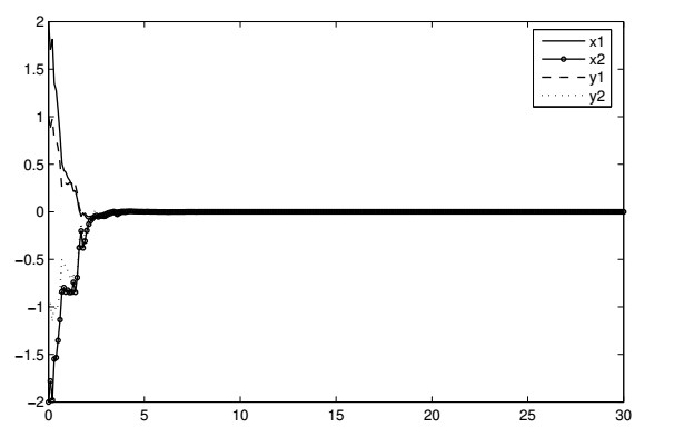
In this research, a non-fragile synchronization of bidirectional association memory (BAM) delayed neural networks is taken into consideration. The controller gain fluctuation seems in a very random manner, that obeys sure Bernoulli distributed noise sequences. Delay dependent criteria are derived to confirm the asymptotic stability of the BAM delayed neural networks. The non-fragile controller are often obtained by determination a collection of linear matrix inequalities (LMIs). A simulation example is used to demonstrate the efficiency of the developed control.
Citation: Ganesh Kumar Thakur, Sudesh Kumar Garg, Tej Singh, M. Syed Ali, Tarun Kumar Arora. Non-fragile synchronization of BAM neural networks with randomly occurring controller gain fluctuation[J]. Mathematical Biosciences and Engineering, 2023, 20(4): 7302-7315. doi: 10.3934/mbe.2023317
In this research, a non-fragile synchronization of bidirectional association memory (BAM) delayed neural networks is taken into consideration. The controller gain fluctuation seems in a very random manner, that obeys sure Bernoulli distributed noise sequences. Delay dependent criteria are derived to confirm the asymptotic stability of the BAM delayed neural networks. The non-fragile controller are often obtained by determination a collection of linear matrix inequalities (LMIs). A simulation example is used to demonstrate the efficiency of the developed control.

| [1] | S. Haykin, Neural Networks: A Comprehensive Foundation, Prentice Hall, New York, 1994. |
| [2] |
Y. Jiang, X. Li, Broadband cancellation method in an adaptive co-site interference cancellation system, Int. J. Electron., 109 (2022), 854–874. https://doi.org/10.1080/00207217.2021.1941295 doi: 10.1080/00207217.2021.1941295

|
| [3] |
R. Ye, P. Liu, K. Shi, B. Yan, State damping control: A novel simple method of rotor UAV with high performance, IEEE Access, 8 (2020), 214346–214357. https://doi.org/10.1109/ACCESS.2020.3040779 doi: 10.1109/ACCESS.2020.3040779
|
| [4] |
K. Liu, F. Ke, X. Huang, R. Yu, F. Lin, Y. Wu, et al., DeepBAN: A temporal convolution-based communication framework for dynamic WBANs, IEEE Trans. Commun., 69 (2021), 6675–6690. https://doi.org/10.1109/TCOMM.2021.3094581 doi: 10.1109/TCOMM.2021.3094581
|
| [5] |
C. Huang, F. Jiang, Q. Huang, X. Wang, Z. Han, W. Huang, Dual-graph attention convolution network for 3-D point cloud classification, IEEE Trans. Neural Networks Learn. Syst., 2022 (2022), 1–13. https://doi.org/10.1109/TNNLS.2022.3162301 doi: 10.1109/TNNLS.2022.3162301
|
| [6] |
K. Liu, Z. Yang, W. Wei, B. Gao, D. Xin, C. Sun, et al., Novel detection approach for thermal defects: Study on its feasibility and application to vehicle cables, High Voltage, 2022 (2022), 1–10. https://doi.org/10.1049/hve2.12258 doi: 10.1049/hve2.12258
|
| [7] |
S. Xu, J. Lam, W. C. Ho, Y. Zou, Delay-dependent exponential stability for a class of neural networks with time delays, J. Comput. Appl. Math., 183 (2005), 16–28. https://doi.org/10.1016/j.cam.2004.12.025 doi: 10.1016/j.cam.2004.12.025
|
| [8] |
O. M. Kwon, S. M. Lee, J. H. Park, E. J. Cha, New approaches on stability criteria for neural networks with interval time-varying delays, Appl. Math. Comput., 218 (2012), 9953–9964. https://doi.org/10.1016/j.amc.2012.03.082 doi: 10.1016/j.amc.2012.03.082
|
| [9] |
S. Arik, An improved robust stability result for uncertain neural networks with multiple time delays, Neural Netw., 54 (2014), 1–10. https://doi.org/10.1016/j.neunet.2014.02.008 doi: 10.1016/j.neunet.2014.02.008
|
| [10] |
J. Y. Zhang, H. Tang, K. Wang, K. Xu, ASRO-DIO: Active subspace random optimization based depth inertial odometry, IEEE Trans. Rob., 2022 (2022), 1–13. https://doi.org/10.1109/TRO.2022.3208503 doi: 10.1109/TRO.2022.3208503
|
| [11] | Q. She, R. Hu, J. Xu, M. Liu, K. Xu, H. Huang, Learning high-DOF reaching-and-grasping via dynamic representation of Gripper-Object, interaction, ACM Trans. Graph., 41 (2022). |
| [12] |
H. Zhao, C. Zhu, X. Xu, H. Huang, K. Xu, Learning practically feasible policies for online 3D bin packing, Sci. China Inf. Sci., 65 (2021), 15–32. https://doi.org/10.1007/s11432-021-3348-6 doi: 10.1007/s11432-021-3348-6
|
| [13] | T. W. Jiang, S. Gong, Highly selective frequency selective surface with ultrawideband rejection, IEEE Trans. Antennas Propag., 70 (2022), 3459–3468. |
| [14] | G. Luo, Q. Yuan, J. Li, S. Wang, F. Yang, Artificial intelligence powered mobile networks: From cognition to decision, IEEE Network, 36 (2022), 136–144. |
| [15] | N. Gunasekaran, N. M. Thoiyab, Q. Zhu, J. Cao, P. Muruganantham, New global asymptotic robust stability of dynamical delayed neural networks via intervalized interconnection matrices IEEE Trans. Cybern., 52 (2022), 11794–11804. |
| [16] | N. M. Thoiyab, P. Muruganantham, Q. Zhu, N. Gunasekaran, Novel results on global stability analysis for multiple time-delayed BAM neural networks under parameter uncertainties, Chaos, Solitons Fractals, 152 (2021), 111441. |
| [17] | N. Gunasekaran, G. Zhai, Q. Yu, Sampled-data synchronization of delayed multi-agent networks and its application to coupled circuit, Neurocomputing, 413 (2020), 499–511. |
| [18] | H. B. Zeng, Y. He, M. Wu, C. F. Zhang, Complete delay–decomposing approach to asymptotic stability for neural networks with time-varying delays, IEEE Trans. Neural Netw., 22 (2011), 806–812. |
| [19] |
Y. Liu, S. M. Lee, O. M. Kwon, J. H. Park, New approach to stability criteria for generalized neural networks with interval time–varying delays, Neurocomputing, 149 (2015), 1544–1551. https://doi.org/10.1016/j.neucom.2014.08.038 doi: 10.1016/j.neucom.2014.08.038
|
| [20] |
S. Arik, An analysis of stability of neutral-type neural systems with constant time delays, J. Franklin Inst., 351 (2014), 4949–4959. https://doi.org/10.1016/j.jfranklin.2014.08.013 doi: 10.1016/j.jfranklin.2014.08.013
|
| [21] |
X. Li, S. Song, Stabilization of delay systems: Delay-dependent impulsive control, IEEE Trans. Autom. Control, 62 (2017), 406–411. https://doi.org/10.1109/TAC.2016.2530041 doi: 10.1109/TAC.2016.2530041
|
| [22] |
X. Li, X. Zhang, S. Song, Effect of delayed impulses on input-to-state stability of nonlinear systems, Automatica, 76 (2017), 378–382. https://doi.org/10.1016/j.automatica.2016.08.009 doi: 10.1016/j.automatica.2016.08.009
|
| [23] |
X. Li, M. Bohner, C. Wang, Impulsive differential equations: Periodic solutions and applications, Automatica, 52 (2015), 173–178. https://doi.org/10.1016/j.automatica.2014.11.009 doi: 10.1016/j.automatica.2014.11.009
|
| [24] |
M. S. Ali, R. Saravanakumar, Q. Zhu, Less conservative delay-dependent $H_\infty$ control of uncertain neural networks with discrete interval and distributed time-varying delays, Neurocomputing, 166 (2015), 84–95. https://doi.org/10.1016/j.neucom.2015.04.023 doi: 10.1016/j.neucom.2015.04.023
|
| [25] |
M. J. Park, O. M. Kwon, J. H. Park, S. M. Lee, A new augmented Lyapunov-Krasovskii functional approach for stability of linear systems with time-varying delays, Appl. Math. Comput., 217 (2011), 7197–7209. https://doi.org/10.1016/j.amc.2011.02.006 doi: 10.1016/j.amc.2011.02.006
|
| [26] |
B. Kosko, Adaptive bidirectional associative memories, Appl. Opt., 26 (1987), 4947–4960. https://doi.org/10.1364/AO.26.004947 doi: 10.1364/AO.26.004947
|
| [27] |
K. Gopalsamy, X. Z. He, Delay independent stability in bidirectional associative memory networks, IEEE Trans. Neural Netw., 5 (1994), 998–1002. https://doi.org/10.1109/72.329700 doi: 10.1109/72.329700
|
| [28] |
J. Cao, G. Stamov, I. Stamova, S. Simeonov, Almost periodicity in impulsive fractional-order reaction-diffusion neural networks with time-varying delays, IEEE Trans. Cybern., 51 (2021), 151–161. https://doi.org/10.1109/TCYB.2020.2967625 doi: 10.1109/TCYB.2020.2967625
|
| [29] |
Y. Wang, X. Hu, K. Shi, X. Song, H. Shen, Network-based passive estimation for switched complex dynamical networks under persistent dwell-time with limited signals, J. Franklin Inst., 3657 (2020), 10921–10936. https://doi.org/10.1016/j.jfranklin.2020.08.037 doi: 10.1016/j.jfranklin.2020.08.037
|
| [30] | M. S. Ali, L. Palanisamy, N. Gunasekaran, A. Alsaedi, B. Ahmad, Finite-time exponential synchronization of reaction-diffusion delayed complex-dynamical networks, Discrete Contin. Dyn. Syst., 14 (2021), 1465. |
| [31] | N. Padmaja, P. Balasubramaniam, Mixed $H_{\infty}$/passivity based stability analysis of fractional-order gene regulatory networks with variable delays, Math. Comput. Simul., 192 (2021), 167–181. |
| [32] |
J. Cao, M. Dong, Exponential stability of delayed bi-directional associative memory networks, Appl. Math. Comput., 135 (2003), 105–112. https://doi.org/10.1016/S0096-3003(01)00315-0 doi: 10.1016/S0096-3003(01)00315-0
|
| [33] |
S. Arik, Global asymptotic stability of bidirectional associative memory neural networks with time delays, IEEE Trans. Neural Netw., 16 (2005), 580–586. https://doi.org/10.1109/TNN.2005.844910 doi: 10.1109/TNN.2005.844910
|
| [34] |
S. Senan, S. Arik, Global robust stability of bidirectional associative memory neural networks with multiple time delays, IEEE Trans. Syst. Man Cybern B., 37 (2007) 1375–1381. https://doi.org/10.1109/TSMCB.2007.902244 doi: 10.1109/TSMCB.2007.902244
|
| [35] |
J. Cao, Y. Wan, Matrix measure strategies for stability and synchronization of inertial BAM neural network with time delays, Neural Netw., 53 (2014), 165–172. https://doi.org/10.1016/j.neunet.2014.02.003 doi: 10.1016/j.neunet.2014.02.003
|
| [36] |
J. Cao, Q. Song, Stability in Cohen–Grossberg-type bidirectional associative memory neural networks with time-varying delays, Nonlinearity, 19 (2006), 1601–1617. https://doi.org/10.1088/0951-7715/19/7/008 doi: 10.1088/0951-7715/19/7/008
|
| [37] |
M. S. Ali, P. Balasubramaniam, Global exponential stability of uncertain fuzzy BAM neural networks with time-varying delays, Chaos, Solitons Fractals, 42 (2009), 2191–2199. https://doi.org/10.1016/j.chaos.2009.03.138 doi: 10.1016/j.chaos.2009.03.138
|
| [38] |
H. Bao, J. Cao, Robust state estimation for uncertain stochastic bidirectional associative memory networks with time-varying delays, Phys. Scripta, 83 (2011), 065004. https://doi.org/10.1088/0031-8949/83/06/065004 doi: 10.1088/0031-8949/83/06/065004
|
| [39] |
K. Mathiyalagan, R. Sakthivel, S. Marshal Anthoni, New robust passivity criteria for stochastic fuzzy BAM neural networks with time-varying delays, Commun. Nonlinear Sci. Numer. Simulat., 17 (2012), 1392–1407. https://doi.org/10.1016/j.cnsns.2011.07.032 doi: 10.1016/j.cnsns.2011.07.032
|
| [40] |
H. Bao, J. Cao, Exponential stability for stochastic BAM networks with discrete and distributed delays, Appl. Math. Comput., 218 (2012), 6188–6199. https://doi.org/10.1016/j.amc.2011.11.035 doi: 10.1016/j.amc.2011.11.035
|
| [41] |
M. S. Ali, R. Saravanakumar, J. Cao, New passivity criteria for memristor-based neutral-type stochastic BAM neural networks with mixed time-varying delays, Neurocomputing, 171 (2016), 1533–1547. https://doi.org/10.1016/j.neucom.2015.07.101 doi: 10.1016/j.neucom.2015.07.101
|
| [42] |
Z. Cai, L. Huang, Functional differential inclusions and dynamic behaviours for memristor-based BAM neural networks with time varying delays, Commun. Nonlinear Sci. Numer. Simulat., 19 (2014), 1279–1300. https://doi.org/10.1016/j.cnsns.2013.09.004 doi: 10.1016/j.cnsns.2013.09.004
|
| [43] |
H. Li, H. Jiang, C. Hu, Existence and global exponential stability of periodic solution of memristor-based BAM neural networks with time-varying delays, Neural Netw., 75 (2016), 97–109. https://doi.org/10.1016/j.neunet.2015.12.006 doi: 10.1016/j.neunet.2015.12.006
|
| [44] |
J. Qi, C. Li, T. Huang, Stability of interval BAM neural network with time varying delay via impulsive control, Neurocomputing, 161 (2015), 162–167. https://doi.org/10.1016/j.neucom.2015.02.052 doi: 10.1016/j.neucom.2015.02.052
|
| [45] |
M. Fang, J. H. Park, Non-fragile synchronization of neural networks with time-varying delay and randomly occurring controller gain fluctuation, Appl. Math. Comput., 219 (2013), 8009–8017. https://doi.org/10.1016/j.amc.2013.02.030 doi: 10.1016/j.amc.2013.02.030
|
| [46] |
Z. G. Wu, J. H. Park, H. Su, J. Chu, Non-fragile synchronization control for complex networks with missing data, Int. J. Control, 86 (2013), 555–566. https://doi.org/10.1080/00207179.2012.747704 doi: 10.1080/00207179.2012.747704
|
| [47] |
R. Rakkiyappan, A. Chandrasekar, G. Petchimmal, Non-fragile robust synchronization for Markovian Jumping choatic neural networks of natural type with randomly occuring uncertainities and mode-dependent time varying delays, ISA Trans., 53 (2014), 1760–1770. https://doi.org/10.1016/j.isatra.2014.09.022 doi: 10.1016/j.isatra.2014.09.022
|
| [48] |
D. Li, Z. Wang, G. Ma, C. Ma, Non-fragile synchronization of dynamical networks with randomly occurring non linearities and controller gain fluctuations, Neurocomputing, 168 (2015), 719–725. https://doi.org/10.1016/j.neucom.2015.05.052 doi: 10.1016/j.neucom.2015.05.052
|
| [49] |
T. H. Lee, J. H. Park, S. M. Lee, O. M. Kwon, Robust synchronisation of chaotic systems with randomly occurring uncertainties via stochastic sampled-data control, Int. J. Control, 86 (2013), 107–119. https://doi.org/10.1080/00207179.2012.720034 doi: 10.1080/00207179.2012.720034
|
| [50] |
R. Anbuvithya, K. Mathiyalagan, R. Sakthivel, P. Prakash, Non-fragile synchronization of Memristive BAM networks with random feedback gain fluctuations, Commun. Nonlinear Sci. Numer. Simulat., 29 (2015), 427–440. https://doi.org/10.1016/j.cnsns.2015.05.020 doi: 10.1016/j.cnsns.2015.05.020
|
| [51] | J. Ren, Q. Zhang, Non-fragile PD state $H_\infty$ control for a class of uncertain descriptor systems, Appl. Math. Comput., 218 (2012), 8806–8815. |
| [52] |
F. Yang, H. Dong, Z. Wang, W. Ren, F. E. Alsaadi, A new approach to non-fragile state estimation for continuous neural network with time delays, Neurocomputing, 197 (2016), 205–211. https://doi.org/10.1016/j.neucom.2016.02.062 doi: 10.1016/j.neucom.2016.02.062
|
| [53] | B. Boyd, L. Ghoui, E. Feron, V. Balakrishnan, Linear Matrix Inequalities in System and Control Theory, Philadephia, PA: SIAM, 1994. https: //doi.org/10.1137/1.9781611970777 |
| [54] | K. Gu, An integral inequality in the stability problem of time-delay systems, in Proceedings of the 39th IEEE Conference on Decision and Control, Sydney, Australia, (2000), 2805–2810. https: //doi.org/10.1109/CDC.2000.914233 |
| [55] |
M. V. Thuan, H. Trinh, L. V. Hien, New inequality-based approach to passivity analysis of neural networks with interval time-varying delay, Neurocomputing, 194 (2016), 301–307. https://doi.org/10.1016/j.neucom.2016.02.051 doi: 10.1016/j.neucom.2016.02.051
|
Figures(1)

Ganesh Kumar Thakur, Sudesh Kumar Garg, Tej Singh, M. Syed Ali, Tarun Kumar Arora. Non-fragile synchronization of BAM neural networks with randomly occurring controller gain fluctuation[J]. Mathematical Biosciences and Engineering, 2023, 20(4): 7302-7315. doi: 10.3934/mbe.2023317


 DownLoad: