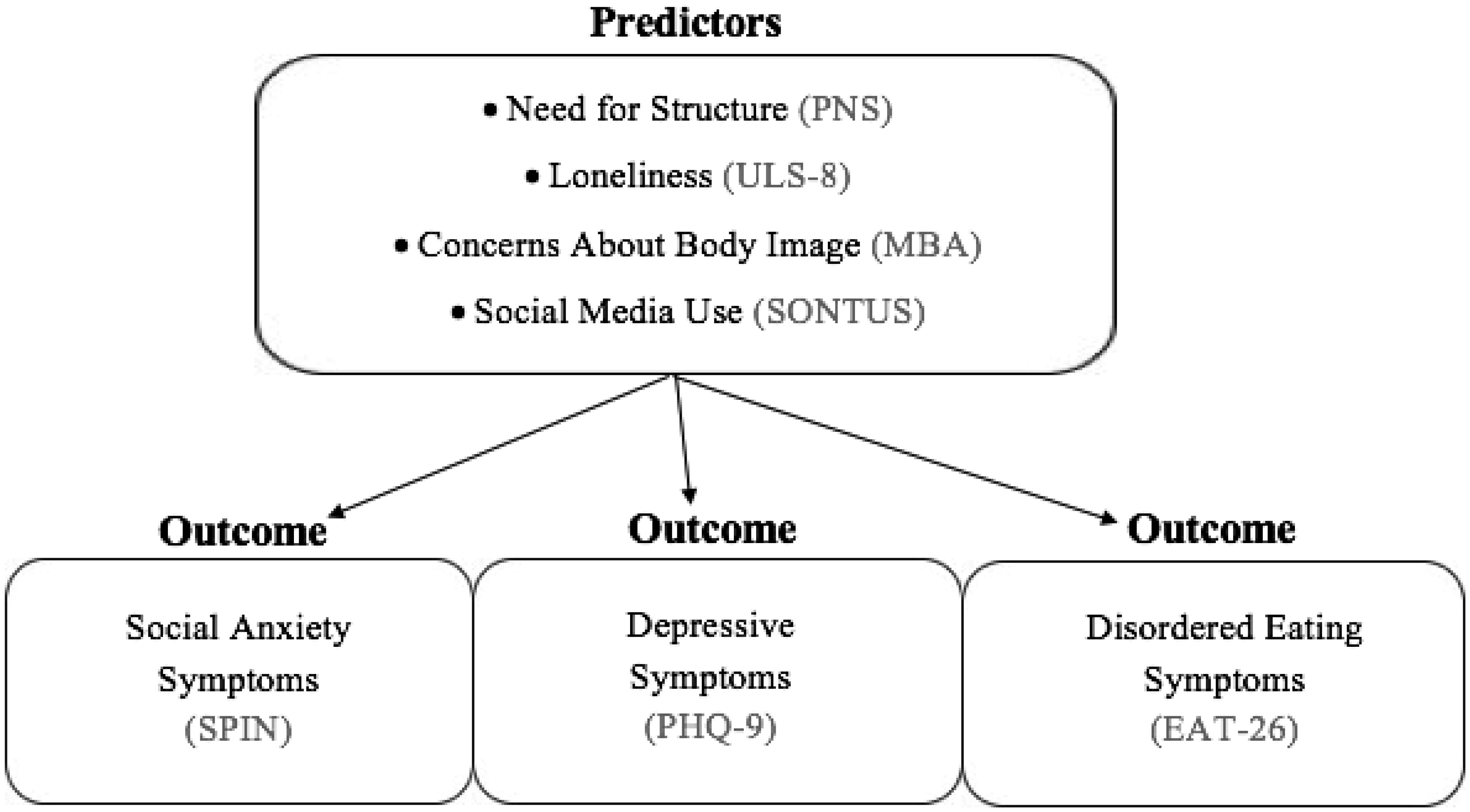
The coronavirus (COVID-19) pandemic has disrupted society and negatively impacted mental health. Various psychosocial risk factors have been exacerbated during the pandemic, leading to the worsening of psychological distress. Specifically, a need for structure, loneliness, concerns about body image and social media use are risk factors previously implicated in poor mental health. The current study examines how these risk factors are associated with mental health outcomes (i.e., social anxiety, depressive and disordered eating symptoms) during the COVID-19 pandemic (January–March 2021). A total of 239 participants were recruited (average age = 24.74, 79% female, 68% White). The results revealed that a need for structure, loneliness and social media use were positively associated with social anxiety. In addition, loneliness, negative concerns about body image and social media use were significantly related to disordered eating and depressive symptoms. Lastly, when examined all together, the overall model for risk factors predicting mental health outcomes was significant: Wilks' Λ = 0.464, F(12, 608.814) = 17.081, p < 0.001. Loneliness and social media use were consistently associated with all psychological symptoms. These results emphasize the need for interventions for social anxiety, depressive and disordered eating symptoms that encourage structured daily activities, social connection, positive perception of oneself and mindful social media use.
Citation: Carlee Bellapigna, Zornitsa Kalibatseva. Psychosocial risk factors associated with social anxiety, depressive and disordered eating symptoms during COVID-19[J]. AIMS Public Health, 2023, 10(1): 18-34. doi: 10.3934/publichealth.2023003
The coronavirus (COVID-19) pandemic has disrupted society and negatively impacted mental health. Various psychosocial risk factors have been exacerbated during the pandemic, leading to the worsening of psychological distress. Specifically, a need for structure, loneliness, concerns about body image and social media use are risk factors previously implicated in poor mental health. The current study examines how these risk factors are associated with mental health outcomes (i.e., social anxiety, depressive and disordered eating symptoms) during the COVID-19 pandemic (January–March 2021). A total of 239 participants were recruited (average age = 24.74, 79% female, 68% White). The results revealed that a need for structure, loneliness and social media use were positively associated with social anxiety. In addition, loneliness, negative concerns about body image and social media use were significantly related to disordered eating and depressive symptoms. Lastly, when examined all together, the overall model for risk factors predicting mental health outcomes was significant: Wilks' Λ = 0.464, F(12, 608.814) = 17.081, p < 0.001. Loneliness and social media use were consistently associated with all psychological symptoms. These results emphasize the need for interventions for social anxiety, depressive and disordered eating symptoms that encourage structured daily activities, social connection, positive perception of oneself and mindful social media use.

| [1] |
Haliwa I, Wilson J, Lee J, et al. (2021) Predictors of change in mental health during the COVID-19 pandemic. J Affect Disord 291: 331-337. https://doi.org/10.1016/j.jad.2021.05.045 
|
| [2] |
Ernst M, Niederer D, Werner AM, et al. (2022) Loneliness before and during the COVID-19 pandemic: A systematic review with meta-analysis. Am Psychol 77: 660-677. https://doi.org/10.1037/amp0001005
|
| [3] |
Palgi Y, Shrira A, Ring L, et al. (2020) The loneliness pandemic: Loneliness and other concomitants of depression, anxiety and their comorbidity during the COVID-19 outbreak. J Affect Disord 275: 109-111. https://doi.org/10.1016/j.jad.2020.06.036
|
| [4] |
McQuaid RJ, Cox SM, Ogunlana A, et al. (2021) The burden of loneliness: Implications of the social determinants of health during COVID-19. Psychiatry Res 296: 113648. https://doi.org/10.1016/j.psychres.2020.113648
|
| [5] |
Choukas-Bradley S, Maheux AJ, Roberts SR, et al. (2022) Picture perfect during a pandemic? Body image concerns and depressive symptoms in US adolescent girls during the COVID-19 lockdown. J Child Media 16: 481-492. https://doi.org/10.1080/17482798.2022.2039255
|
| [6] |
Nutley SK, Falise AM, Henderson R, et al. (2021) Impact of the COVID-19 pandemic on disordered eating behavior: Qualitative analysis of social media posts. JMIR Ment Health 8: e26011. https://doi.org/10.2196/26011
|
| [7] |
Lee Y, Jeon YJ, Kang S, et al. (2022) Social media use and mental health during the COVID-19 pandemic in young adults: a meta-analysis of 14 cross-sectional studies. BMC Public Health 22: 995. https://doi.org/10.1186/s12889-022-13409-0
|
| [8] |
Safieh J, Broughan J, McCombe G, et al. (2022) Interventions to optimise mental health outcomes during the COVID-19 pandemic: A scoping review. Int J Ment Health Addict 20: 2934-2955. https://doi.org/10.1007/s11469-021-00558-3
|
| [9] |
Sousa GMD, Tavares VDDO, de Meiroz Grilo MLP, et al. (2021) Mental health in COVID-19 pandemic: a meta-review of prevalence meta-analyses. Front Psychol 12: 703838. https://doi.org/10.3389/fpsyg.2021.703838
|
| [10] | Prokopčáková A (2015) Personal need for structure, anxiety, self-efficacy and optimism. Stud Psychol 57: 147-162. https://doi.org/10.21909/sp.2015.02.690 |
| [11] |
Cacioppo S, Grippo US, London S, et al. (2015) Loneliness: Clinical import and interventions. Perspect Psychol Sci 10: 238-249. https://doi.org/10.1177/1745691615570616
|
| [12] | Manaf NA, Saravanan C, Zuhrah B (2016) The prevalence and inter-relationship of negative body image perception, depression and susceptibility to eating disorders among female medical undergraduate students. J Clin Diagn Res 10: VC01-VC04. https://doi.org/10.7860/JCDR/2016/16678.7341 |
| [13] |
Twenge JM (2019) More time on technology, less happiness? Associations between digital-media use and psychological well-being. Curr Dir Psychol Sci 28: 372-379. https://doi.org/10.1177/0963721419838244
|
| [14] |
Adams GC, Balbuena L, Meng X, et al. (2016) When social anxiety and depression go together: A population study of comorbidity and associated consequences. J Affect Disord 206: 48-54. https://doi.org/10.1016/j.jad.2016.07.031
|
| [15] |
Garcia SC, Mikhail ME, Keel PK, et al. (2020) Increased rates of eating disorders and their symptoms in women with major depressive disorder and anxiety disorders. Int J Eat Disord 53: 1844-1854. https://doi.org/10.1002/eat.23366
|
| [16] |
Bueno-Notivol J, Gracia-García P, Olaya B, et al. (2021) Prevalence of depression during the COVID-19 outbreak: A meta-analysis of community-based studies. Int J Clin Health Psychol 21: 100196-100211. https://doi.org/10.1016/j.ijchp.2020.07.007
|
| [17] |
Li Y, Zhao J, Ma Z, et al. (2021) Mental health among college students during the COVID-19 pandemic in China: A 2-wave longitudinal survey. J Affect Disord 281: 597-604. https://doi.org/10.1016/j.jad.2020.11.109
|
| [18] | National Institute of Mental HealthDepression (2018). Available from: https://www.nimh.nih.gov/health/topics/depression. |
| [19] | American Psychiatric AssociationDiagnostic and statistical manual of mental disorders (5th ed.) (2013). https://doi.org/10.1176/appi.books.9780890425596 |
| [20] |
Hawes MT, Szenczy AK, Klein DN, et al. (2021) Increases in depression and anxiety symptoms in adolescents and young adults during the COVID-19 pandemic. Psychol Med 52: 3222-3230. https://doi.org/10.1017/S0033291720005358
|
| [21] |
Abebe DS, Torgersen L, Lien L, et al. (2014) Predictors of disordered eating in adolescence and young adulthood: A population-based, longitudinal study of females and males in Norway. Int J Behav Dev 38: 128-138. https://doi.org/10.1177/0165025413514871
|
| [22] |
Ramalho SM, Trovisqueira A, de Lourdes M, et al. (2021) The impact of COVID-19 lockdown on disordered eating behaviors: The mediation role of psychological distress. Eat Weight Disord 27: 179-188. https://doi.org/10.1007/s40519-021-01128-1
|
| [23] |
McLean CP, Utpala R, Sharp G (2022) The impacts of COVID-19 on eating disorders and disordered eating: A mixed studies systematic review and implications. Front Psychol 13: 926709. https://doi.org/10.3389/fpsyg.2022.926709
|
| [24] |
Fernández-Aranda F, Casas M, Claes L, et al. (2020) COVID-19 and implications for eating disorders. Eur Eat Disord Rev 28: 239-245. https://doi.org/10.1002/erv.2738
|
| [25] |
Arad G, Shamai-Leshem D, Bar-Haim Y (2021) Social distancing during a COVID-19 lockdown contributes to the maintenance of social anxiety: a natural experiment. Cognit Ther Res 45: 708-714. https://doi.org/10.1007/s10608-021-10231-7
|
| [26] | National Institute of Mental HealthAnxiety disorders (2018). Available from: https://www.nimh.nih.gov/health/topics/anxiety-disorders. |
| [27] |
Beard C, Amir N (2009) Interpretation in social anxiety: When meaning precedes ambiguity. Cognit Ther Res 33: 406-415. https://doi.org/10.1007/s10608-009-9235-0
|
| [28] |
Olivera-La Rosa A, Chuquichambi EG, Ingram GP (2020) Keep your (social) distance: Pathogen concerns and social perception in the time of COVID-19. Pers Individ Dif 166: 110200. https://doi.org/10.1016/j.paid.2020.110200
|
| [29] |
Hwang TJ, Rabheru K, Peisah C, et al. (2020) Loneliness and social isolation during the COVID-19 pandemic. Int Psychogeriatr 32: 1217-1220. https://doi.org/10.1017/S1041610220000988
|
| [30] |
Neuberg SL, Newsom J T (1993) Personal need for structure: Individual differences in the desire for simpler structure. J Pers Soc Psychol 65: 113-131. https://doi.org/10.1037/0022-3514.65.1.113
|
| [31] |
Giuntella O, Hyde K, Saccardo S, et al. (2021) Lifestyle and mental health disruptions during COVID-19. Proc Natl Acad Sci 118: e2016632118. https://doi.org/10.1073/pnas.2016632118
|
| [32] |
Rodgers RF, Lombardo C, Cerolini S, et al. (2020) The impact of the COVID-19 pandemic on eating disorder risk and symptoms. Int J Eat Disord 53: 1166-1170. https://doi.org/10.1002/eat.23318
|
| [33] |
Lim MH, Rodebaugh TL, Zyphur MJ, et al. (2016) Loneliness over time: The crucial role of social anxiety. J Abnorm Psychol 125: 620-630. https://doi.org/10.1037/abn0000162
|
| [34] |
Van der Velden PG, Hyland P, Contino C, et al. (2021) Anxiety and depression symptoms, the recovery from symptoms, and loneliness before and after the COVID-19 outbreak among the general population: Findings from a Dutch population-based longitudinal study. PloS One 16: e0245057. https://doi.org/10.1371/journal.pone.0245057
|
| [35] |
Aderka IM, Gutner CA, Lazarov A, et al. (2013) Body image in social anxiety disorder, obsessive-compulsive disorder, and panic disorder. Body Image 11: 51-56. https://doi.org/10.1016/j.bodyim.2013.09.002
|
| [36] |
Grogan S (2006) Body Image and Health: Contemporary Perspectives. J Health Psychol 11: 523-530. https://doi.org/10.1177/1359105306065013
|
| [37] |
Swami S, Tran US, Stieger S, et al. (2015) Associations between women's body image and happiness: Results of the youbeauty.com body image survey (YBIS). J Happiness Stud 16: 705-718. https://doi.org/10.1007/s10902-014-9530-7
|
| [38] |
Bucchianeri MM, Arikian AJ, Hannan PJ, et al. (2013) Body dissatisfaction from adolescence to young adulthood: Findings from a 10-year longitudinal study. Body Image 10: 1-7. https://doi.org/10.1016/j.bodyim.2012.09.001
|
| [39] |
Dakanalis A, Carrà G, Calogero R, et al. (2015) The developmental effects of media-ideal internalization and self-objectification processes on adolescents' negative body-feelings, dietary restraint, and binge eating. Eur Child Adolesc Psychiatry 24: 997-1010. https://doi.org/10.1007/s00787-014-0649-1
|
| [40] |
Sherman LE, Greenfield PM, Hernandez LM, et al. (2017) Peer influence via Instagram: Effects on brain and behavior in adolescence and young adulthood. Child Dev 89: 37-47. https://doi.org/10.1111/cdev.12838
|
| [41] | Thompson MM, Naccarato ME, Parker KCH, et al. (2001) The Personal Need for Structure (PNS) and Personal Fear of Invalidity (PFI) scales: Historical perspectives, present applications and future directions. Cognitive Social Psychology: The Princeton Symposium on the Legacy and Future of Social Cognition . Mahwah, NJ: Erlbaum 19-39. |
| [42] |
Hays RD, DiMatteo MR (1987) A short-form measure of loneliness. J Pers Assess 51: 69-81. https://doi.org/10.1207/s15327752jpa5101_6
|
| [43] |
Carver CS, Pozo-Kaderman C, Price AA, et al. (1998) Concern about aspects of body image and adjustment to early stage breast cancer. J Psychosom Med 60: 168-174. https://doi.org/10.1097/00006842-199803000-00010
|
| [44] |
Olufadi Y (2016) Social networking time use scale (SONTUS): A new instrument for measuring the time spent on the social networking sites. Telemat Inform 33: 452-471. https://doi.org/10.1016/j.tele.2015.11.002
|
| [45] |
Garner DM, Olmsted MP, Bohr Y, et al. (1982) The eating attitudes test: Psychometric features and clinical correlates. Psychol Med 12: 871-878. https://doi.org/10.1017/s0033291700049163
|
| [46] |
Connor K, Davidson J, Churchill L, et al. (2000) Psychometric properties of the Social Phobia Inventory (SPIN): New self-rating scale. Br J Psychiatry 176: 379-386. https://doi.org/10.1192/bjp.176.4.379
|
| [47] |
Kroenke K, Spitzer R, Williams J (2001) The PHQ-9: Validity of a brief depression severity measure. J Gen Intern Med 16: 606-613. https://doi.org/10.1046/j.1525-1497.2001.016009606.x
|
| [48] |
Cooper M, Reilly EE, Siegel JA, et al. (2020) Eating disorders during the COVID-19 pandemic and quarantine: An overview of risks and recommendations for treatment and early interventions. Eat Disord 30: 54-76. https://doi.org/10.1080/10640266.2020.1790271
|
| [49] |
Haines J, Kleinman KP, Rifas-Shiman SL, et al. (2010) Examination of shared risk and protective factors for overweight and disordered eating among adolescents. Arch Pediatr Adolesc Med 164: 336-343. https://doi.org/10.1001/archpediatrics.2010.19
|
| [50] |
Ge L, Yap CW, Ong R, et al. (2017) Social isolation, loneliness and their relationships with depressive symptoms: A population-based study. PloS One 12: e0182145. https://doi.org/10.1371/journal.pone.0182145
|
| [51] | Center for Disease Control and PreventionCoping with stress (2020). Available from: https://www.cdc.gov/mentalhealth/stress-coping/cope-with-stress/index.html. |
Figures(1) / Tables(3)

Carlee Bellapigna, Zornitsa Kalibatseva. Psychosocial risk factors associated with social anxiety, depressive and disordered eating symptoms during COVID-19[J]. AIMS Public Health, 2023, 10(1): 18-34. doi: 10.3934/publichealth.2023003


 DownLoad: