Investigating the effect of changes in neuronal connectivity on the brain's behavior is of interest in neuroscience studies. Complex network theory is one of the most capable tools to study the effects of these changes on collective brain behavior. By using complex networks, the neural structure, function, and dynamics can be analyzed. In this context, various frameworks can be used to mimic neural networks, among which multi-layer networks are a proper one. Compared to single-layer models, multi-layer networks can provide a more realistic model of the brain due to their high complexity and dimensionality. This paper examines the effect of changes in asymmetry coupling on the behaviors of a multi-layer neuronal network. To this aim, a two-layer network is considered as a minimum model of left and right cerebral hemispheres communicated with the corpus callosum. The chaotic model of Hindmarsh-Rose is taken as the dynamics of the nodes. Only two neurons of each layer connect two layers of the network. In this model, it is assumed that the layers have different coupling strengths, so the effect of each coupling change on network behavior can be analyzed. As a result, the projection of the nodes is plotted for several coupling strengths to investigate how the asymmetry coupling influences the network behaviors. It is observed that although no coexisting attractor is present in the Hindmarsh-Rose model, an asymmetry in couplings causes the emergence of different attractors. The bifurcation diagrams of one node of each layer are presented to show the variation of the dynamics due to coupling changes. For further analysis, the network synchronization is investigated by computing intra-layer and inter-layer errors. Calculating these errors shows that the network can be synchronized only for large enough symmetric coupling.
Citation: Sridevi Sriram, Hayder Natiq, Karthikeyan Rajagopal, Ondrej Krejcar, Hamidreza Namazi. Dynamics of a two-layer neuronal network with asymmetry in coupling[J]. Mathematical Biosciences and Engineering, 2023, 20(2): 2908-2919. doi: 10.3934/mbe.2023137
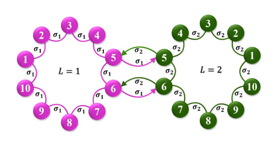
Investigating the effect of changes in neuronal connectivity on the brain's behavior is of interest in neuroscience studies. Complex network theory is one of the most capable tools to study the effects of these changes on collective brain behavior. By using complex networks, the neural structure, function, and dynamics can be analyzed. In this context, various frameworks can be used to mimic neural networks, among which multi-layer networks are a proper one. Compared to single-layer models, multi-layer networks can provide a more realistic model of the brain due to their high complexity and dimensionality. This paper examines the effect of changes in asymmetry coupling on the behaviors of a multi-layer neuronal network. To this aim, a two-layer network is considered as a minimum model of left and right cerebral hemispheres communicated with the corpus callosum. The chaotic model of Hindmarsh-Rose is taken as the dynamics of the nodes. Only two neurons of each layer connect two layers of the network. In this model, it is assumed that the layers have different coupling strengths, so the effect of each coupling change on network behavior can be analyzed. As a result, the projection of the nodes is plotted for several coupling strengths to investigate how the asymmetry coupling influences the network behaviors. It is observed that although no coexisting attractor is present in the Hindmarsh-Rose model, an asymmetry in couplings causes the emergence of different attractors. The bifurcation diagrams of one node of each layer are presented to show the variation of the dynamics due to coupling changes. For further analysis, the network synchronization is investigated by computing intra-layer and inter-layer errors. Calculating these errors shows that the network can be synchronized only for large enough symmetric coupling.

| [1] |
F. Parastesh, S. Jafari, H. Azarnoush, Z. Shahriari, Z. Wang, S. Boccaletti, et al., Chimeras, Phys. Rep., 898 (2021), 1–114. https://doi.org/10.1016/j.physrep.2020.10.003 doi: 10.1016/j.physrep.2020.10.003

|
| [2] |
S. Majhi, B. K. Bera, D. Ghosh, M. Perc, Chimera states in neuronal networks: A review, Phys. Life Rev., 28 (2019), 100–121. https://doi.org/10.1016/j.plrev.2018.09.003 doi: 10.1016/j.plrev.2018.09.003
|
| [3] |
F. Parastesh, M. Mehrabbeik, K. Rajagopal, S. Jafari, M. Perc, Synchronization in Hindmarsh-Rose neurons subject to higher-order interactions, Chaos, 32 (2022), 013125. https://doi.org/10.1063/5.0079834 doi: 10.1063/5.0079834
|
| [4] |
K. Rajagopal, S. He, A. Karthikeyan, P. Duraisamy, Size matters: Effects of the size of heterogeneity on the wave re-entry and spiral wave formation in an excitable media, Chaos, 31 (2021), 053131. https://doi.org/10.1063/5.0051010 doi: 10.1063/5.0051010
|
| [5] |
Z. Wang, Z. Rostami, S. Jafari, F. E. Alsaadi, M. Slavinec, M. Perc, Suppression of spiral wave turbulence by means of periodic plane waves in two-layer excitable media, Chaos Solitons Fractals, 128 (2019), 229–233. https://doi.org/10.1016/j.chaos.2019.07.045 doi: 10.1016/j.chaos.2019.07.045
|
| [6] |
Z. Yao, C. Wang, P. Zhou, J. Ma, Regulating synchronous patterns in neurons and networks via field coupling, Commun. Nonlinear Sci. Numer. Simul., 95 (2021), 105583. https://doi.org/10.1016/j.cnsns.2020.105583 doi: 10.1016/j.cnsns.2020.105583
|
| [7] |
Z. Yao, C. Wang, Control the collective behaviors in a functional neural network, Chaos Solitons Fractals, 152 (2021), 111361. https://doi.org/10.1016/j.chaos.2021.111361 doi: 10.1016/j.chaos.2021.111361
|
| [8] |
P. Zhou, X. Zhang, X. Hu, G. Ren, Energy balance between two thermosensitive circuits under field coupling, Nonlinear Dyn., 110 (2022), 1879–1895. https://doi.org/10.1007/s11071-022-07669-z doi: 10.1007/s11071-022-07669-z
|
| [9] |
N. Naseri, F. Parastesh, F. Ghassemi, S. Jafari, E. Schö ll, J. Kurths, Converting high dimensional complex networks to lower dimensional ones preserving synchronization features, Eur. Lett., 140 (2022), 21001. https://doi.org/10.1209/0295-5075/ac98de doi: 10.1209/0295-5075/ac98de
|
| [10] |
V. Thibeault, G. St-Onge, L. J. Dubé, P. Desrosiers, Threefold way to the dimension reduction of dynamics on networks: An application to synchronization, Phys. Rev. Res., 2 (2020), 043215. https://doi.org/10.1103/PhysRevResearch.2.043215 doi: 10.1103/PhysRevResearch.2.043215
|
| [11] |
Q. Xu, T. Liu, S. Ding, H. Bao, Z. Li, B. Chen, Extreme multistability and phase synchronization in a heterogeneous bi-neuron Rulkov network with memristive electromagnetic induction, Cogn. Neurodyn., 2022 (2022), 1–12. https://doi.org/10.1007/s11571-022-09866-3 doi: 10.1007/s11571-022-09866-3
|
| [12] |
Q. Xu, X. Tan, D. Zhu, M. Chen, J. Zhou, H. Wu, Synchronous behavior for memristive synapse-connected Chay twin-neuron network and hardware implementation, Math. Probl. Eng., 2020 (2022), 8218740. https://doi.org/10.1155/2020/8218740 doi: 10.1155/2020/8218740
|
| [13] |
S. Rakshit, S. Majhi, J. Kurths, D. Ghosh, Neuronal synchronization in long-range time-varying networks, Chaos, 31 (2021), 073129. https://doi.org/10.1063/5.0057276 doi: 10.1063/5.0057276
|
| [14] |
K. Clark, R. F. Squire, Y. Merrikhi, B. Noudoost, Visual attention: Linking prefrontal sources to neuronal and behavioral correlates, Prog. Neurobiol., 132 (2015), 59–80. https://doi.org/10.1016/j.pneurobio.2015.06.006 doi: 10.1016/j.pneurobio.2015.06.006
|
| [15] |
Z. Bahmani, K. Clark, Y. Merrikhi, A. Mueller, W. Pettine, M. I. Vanegas, et al., Prefrontal contributions to attention and working memory, Curr. Top Behav. Neurosci., 41 (2019), 129–153. https://doi.org/10.1007/7854_2018_74 doi: 10.1007/7854_2018_74
|
| [16] |
J. S. Kwon, B. F. O'Donnell, G. V. Wallenstein, R. W. Greene, Y. Hirayasu, P. G. Nestor, et al., Gamma frequency-range abnormalities to auditory stimulation in schizophrenia, Arch. Gen. Psychiatry, 56 (1999), 1001–1005. https://doi.org/10.1001/archpsyc.56.11.1001 doi: 10.1001/archpsyc.56.11.1001
|
| [17] |
G. G. Knyazev, J. Y. Slobodskoj-Plusnin, A. V. Bocharov, L. V. Pylkova, The default mode network and EEG alpha oscillations: An independent component analysis, Brain Res., 1402 (2011), 67–79. https://doi.org/10.1016/j.brainres.2011.05.052 doi: 10.1016/j.brainres.2011.05.052
|
| [18] |
F. A. Fishburn, V. P. Murty, C. O. Hlutkowsky, C. E. MacGillivray, L. M. Bemis, M. E. Murphy, et al., Putting our heads together: interpersonal neural synchronization as a biological mechanism for shared intentionality, Soc. Cogn. Affect. Neurosci., 13 (2018), 841–849. https://doi.org/10.1093/scan/nsy060 doi: 10.1093/scan/nsy060
|
| [19] |
E. Bullmore, O. Sporns, Complex brain networks: Graph theoretical analysis of structural and functional systems, Nat. Rev. Neurosci., 10 (2009), 186–198. https://doi.org/10.1038/nrn2575 doi: 10.1038/nrn2575
|
| [20] |
P. Hagmann, L. Cammoun, X. Gigandet, R. Meuli, C. J. Honey, V. J. Wedeen, et al., Mapping the structural core of human cerebral cortex, PLoS Biol., 6 (2008), e159. https://doi.org/10.1371/journal.pbio.0060159 doi: 10.1371/journal.pbio.0060159
|
| [21] |
B. P. Rogers, V. L. Morgan, A. T. Newton, J. C. Gore, Assessing functional connectivity in the human brain by fMRI, Magn. Reson. Imaging, 25 (2007), 1347–1357. https://doi.org/10.1016/j.mri.2007.03.007 doi: 10.1016/j.mri.2007.03.007
|
| [22] |
M. Gosak, M. Milojević, M. Duh, K. Skok, M. Perc, Networks behind the morphology and structural design of living systems, Phys. Life Rev., 41 (2022), 1–21. https://doi.org/10.1016/j.plrev.2022.03.001 doi: 10.1016/j.plrev.2022.03.001
|
| [23] |
S. D. Glick, D. A. Ross, L. B. Hough, Lateral asymmetry of neurotransmitters in human brain, Brain Res., 234 (1982), 53–63. https://doi.org/10.1016/0006-8993(82)90472-3 doi: 10.1016/0006-8993(82)90472-3
|
| [24] |
L. Tian, J. Wang, C. Yan, Y. He, Hemisphere-and gender-related differences in small-world brain networks: a resting-state functional MRI study, Neuroimage, 54 (2011), 191–202. https://doi.org/10.1016/j.neuroimage.2010.07.066 doi: 10.1016/j.neuroimage.2010.07.066
|
| [25] |
S. F. Witelson, D. L. Kigar, Sylvian fissure morphology and asymmetry in men and women: bilateral differences in relation to handedness in men, J. Comp. Neurol., 323 (1992), 326–340. https://doi.org/10.1002/cne.903230303 doi: 10.1002/cne.903230303
|
| [26] | L. Jäncke, G. Schlaug, Y. Huang, H. Steinmetz, Asymmetry of the planum parietale, Neuroreport, 5 (1994), 1161–1163. https://psycnet.apa.org/doi/10.1097/00001756-199405000-00035 |
| [27] |
G. W. Hynd, M. Semrud-Clikeman, A. R. Lorys, E. S. Novey, D. Eliopulos, Brain morphology in developmental dyslexia and attention deficit disorder/hyperactivity, Arch. Neurol., 47 (1990), 919–926. https://doi.org/10.1001/archneur.1990.00530080107018 doi: 10.1001/archneur.1990.00530080107018
|
| [28] |
R. M. Bilder, H. Wu, B. Bogerts, M. Ashtari, D. Robinson, M. Woerner, et al., Cerebral volume asymmetries in schizophrenia and mood disorders: A quantitative magnetic resonance imaging study, Int. J. Psychophysiol., 34 (1999), 197–205. https://doi.org/10.1016/S0167-8760(99)00077-X doi: 10.1016/S0167-8760(99)00077-X
|
| [29] |
P. M. Thompson, J. Moussai, S. Zohoori, A. Goldkorn, A. A. Khan, M. S. Mega, et al., Cortical variability and asymmetry in normal aging and Alzheimer's disease, Cereb. Cortex, 8 (1998), 492–509. https://doi.org/10.1093/cercor/8.6.492 doi: 10.1093/cercor/8.6.492
|
| [30] |
S. Rakshit, F. Parastesh, S. N. Chowdhury, S. Jafari, J. Kurths, D. Ghosh, Relay interlayer synchronisation: invariance and stability conditions, Nonlinearity, 35 (2021), 681. https://doi.org/10.1088/1361-6544/ac3c2f doi: 10.1088/1361-6544/ac3c2f
|
| [31] |
E. S. Medeiros, U. Feudel, A. Zakharova, Asymmetry-induced order in multilayer networks, Phys. Rev. E, 104 (2021), 024302. https://doi.org/10.1103/PhysRevE.104.024302 doi: 10.1103/PhysRevE.104.024302
|
| [32] |
B. M. Tijms, A. M. Wink, W. de Haan, W. M. van der Flier, C. J. Stam, P. Scheltens, et al., Alzheimer's disease: Connecting findings from graph theoretical studies of brain networks, Neurobiol. Aging, 34 (2013), 2023–2036. https://doi.org/10.1016/j.neurobiolaging.2013.02.020 doi: 10.1016/j.neurobiolaging.2013.02.020
|
| [33] |
S. Majhi, M. Perc, D. Ghosh, Dynamics on higher-order networks: A review, J. R. Soc. Interface, 19 (2022), 20220043. https://doi.org/10.1098/rsif.2022.0043 doi: 10.1098/rsif.2022.0043
|
| [34] |
M. De Domenico, A. Solé-Ribalta, E. Cozzo, M. Kivelä, Y. Moreno, M. A. Porter, et al., Mathematical formulation of multilayer networks, Phys. Rev. X, 3 (2013), 041022. https://doi.org/10.1103/PhysRevX.3.041022 doi: 10.1103/PhysRevX.3.041022
|
| [35] |
F. Battiston, V. Nicosia, M. Chavez, V. Latora, Multilayer motif analysis of brain networks, Chaos, 27 (2017), 047404. https://doi.org/10.1063/1.4979282 doi: 10.1063/1.4979282
|
| [36] |
A. Karthikeyan, I. Moroz, K. Rajagopal, P. Duraisamy, Effect of temperature sensitive ion channels on the single and multilayer network behavior of an excitable media with electromagnetic induction, Chaos Solitons Fractals, 150 (2021), 111144. https://doi.org/10.1016/j.chaos.2021.111144 doi: 10.1016/j.chaos.2021.111144
|
| [37] |
M. Yu, M. M. A. Engels, A. Hillebrand, E. C. W. Van Straaten, A. A. Gouw, C. Teunissen, et al., Selective impairment of hippocampus and posterior hub areas in Alzheimer's disease: An MEG-based multiplex network study, Brain, 140 (2017), 1466–1485. https://doi.org/10.1093/brain/awx050 doi: 10.1093/brain/awx050
|
| [38] |
L. Kang, C. Tian, S. Huo, Z. Liu, A two-layered brain network model and its chimera state, Sci. Rep., 9 (2019), 14389. https://doi.org/10.1038/s41598-019-50969-5 doi: 10.1038/s41598-019-50969-5
|


Figures(6)

Sridevi Sriram, Hayder Natiq, Karthikeyan Rajagopal, Ondrej Krejcar, Hamidreza Namazi. Dynamics of a two-layer neuronal network with asymmetry in coupling[J]. Mathematical Biosciences and Engineering, 2023, 20(2): 2908-2919. doi: 10.3934/mbe.2023137


 DownLoad: