Traditional lectures are commonly understood to be a teacher-centered mode of instruction where the main aim is a provision of explanations by an educator to the students. Recent literature in higher education overwhelmingly depicts this mode of instruction as inferior compared to the desired student-centered models based on active learning techniques. First, using a four-quadrant model of educational environments, we address common confusion related to a conflation of two prevalent dichotomies by focusing on two key dimensions: (1) the extent to which students are prompted to engage actively and (2) the extent to which expert explanations are provided. Second, using a case study, we describe an evolution of tertiary mathematics education, showing how traditional instruction can still play a valuable role, provided it is suitably embedded in a student-centered course design. We support our argument by analyzing the teaching practice and learning environment in a third-year abstract algebra course through the lens of Stanislas Dehaene's theoretical framework for effective teaching and learning. The framework, comprising "four pillars of learning", is based on a state-of-the-art conception of how learning can be facilitated according to cognitive science, educational psychology and neuroscience findings. In the case study, we illustrate how, over time, the unit design and the teaching approach have evolved into a learning environment that aligns with the four pillars of learning. We conclude that traditional lectures can and do evolve to optimize learning environments and that the erection of the dichotomy "traditional instruction versus active learning" is no longer relevant.
Citation: Heiko Dietrich, Tanya Evans. Traditional lectures versus active learning – A false dichotomy?[J]. STEM Education, 2022, 2(4): 275-292. doi: 10.3934/steme.2022017
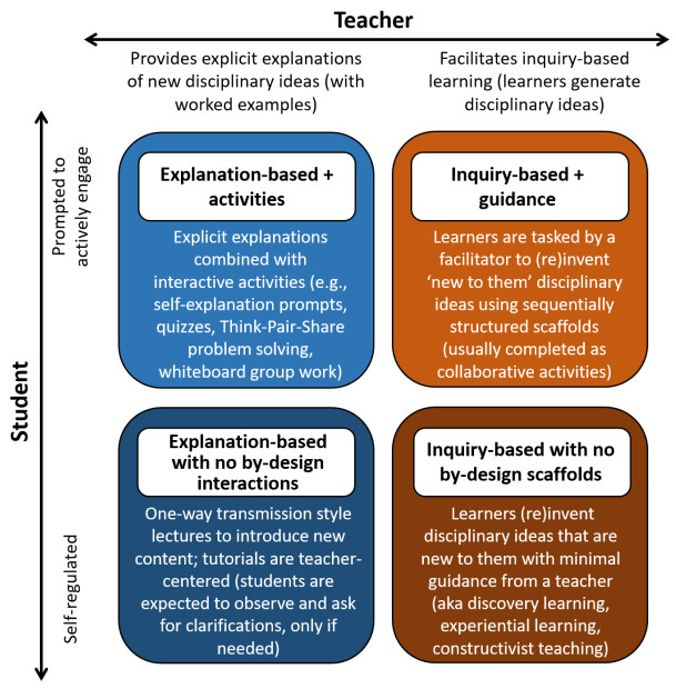
Traditional lectures are commonly understood to be a teacher-centered mode of instruction where the main aim is a provision of explanations by an educator to the students. Recent literature in higher education overwhelmingly depicts this mode of instruction as inferior compared to the desired student-centered models based on active learning techniques. First, using a four-quadrant model of educational environments, we address common confusion related to a conflation of two prevalent dichotomies by focusing on two key dimensions: (1) the extent to which students are prompted to engage actively and (2) the extent to which expert explanations are provided. Second, using a case study, we describe an evolution of tertiary mathematics education, showing how traditional instruction can still play a valuable role, provided it is suitably embedded in a student-centered course design. We support our argument by analyzing the teaching practice and learning environment in a third-year abstract algebra course through the lens of Stanislas Dehaene's theoretical framework for effective teaching and learning. The framework, comprising "four pillars of learning", is based on a state-of-the-art conception of how learning can be facilitated according to cognitive science, educational psychology and neuroscience findings. In the case study, we illustrate how, over time, the unit design and the teaching approach have evolved into a learning environment that aligns with the four pillars of learning. We conclude that traditional lectures can and do evolve to optimize learning environments and that the erection of the dichotomy "traditional instruction versus active learning" is no longer relevant.

| [1] |
Collegiate mathematics teaching in proof-based courses: What we now know and what we have yet to learn. The Journal of Mathematical Behavior (2022) 67: 100986. 
|
| [2] |
Active learning increases student performance in science, engineering, and mathematics. Proceedings of the National Academy of Sciences (2014) 111: 8410-8415.
|
| [3] |
I on the Prize: Inquiry Approaches in Undergraduate Mathematics. International Journal of Research in Undergraduate Mathematics Education (2019) 5: 129-146.
|
| [4] |
Inquiry-based mathematics education: a call for reform in tertiary education seems unjustified. STEM Education (2022) 2: 221-244.
|
| [5] | The act of discovery. Harvard Educational Review (1961) 31: 21-32. |
| [6] |
Bruner, J.S., The art of dicovery, in Understanding Children, M. Sindwani, Ed. 2004. Andrews University: Australian Council for Educational Research. |
| [7] |
Dehaene, S., How We Learn: The New Science of Education and the Brain. 2020: Penguin Books Limited. |
| [8] |
Why Minimal Guidance During Instruction Does Not Work: An Analysis of the Failure of Constructivist, Discovery, Problem-Based, Experiential, and Inquiry-Based Teaching. Educational Psychologist (2006) 41: 75-86.
|
| [9] |
Attentional control of early perceptual learning. Proceedings of the National Academy of Sciences (1993) 90: 5718-5722.
|
| [10] |
Attention: the mechanisms of consciousness. Proceedings of the National Academy of Sciences (1994) 91: 7398-7403.
|
| [11] |
Inattentional blindness: Looking without seeing. Current directions in psychological science (2003) 12: 180-184.
|
| [12] | The influence of retrieval on retention. Memory & cognition (1992) 20: 633-642. |
| [13] |
Test-enhanced learning: Taking memory tests improves long-term retention. Psychological Science (2006) 17: 249-255.
|
| [14] |
Improving Students' Learning With Effective Learning Techniques. Psychological Science in the Public Interest (2013) 14: 4-58.
|
| [15] |
Optimizing distributed practice: theoretical analysis and practical implications. Experimental psychology (2009) 56: 236.
|
| [16] |
Distributed practice in verbal recall tasks: A review and quantitative synthesis. Psychological Bulletin (2006) 132: 354.
|
| [17] |
Dual coding theory and education. Educational Psychology Review (1991) 3: 149-210.
|
| [18] |
Baddeley, A.D. and Hitch, G., Working memory, in Psychology of learning and motivation. 1974, 47‒89. Elsevier. |
| [19] |
Working memory. Science (1992) 255: 556-559.
|
| [20] | Note-taking and handouts in the digital age. American journal of pharmaceutical education (2015) 79:. |
| [21] |
Fiorella, L. and Mayer, R.E., Learning as a generative activity. 2015: Cambridge University Press. |
| [22] |
Problem-solving or Explicit Instruction: Which Should Go First When Element Interactivity Is High?. Educational Psychology Review (2020) 32: 229-247.
|
| [23] |
Self-explanation training improves proof comprehension. Journal for Research in Mathematics Education (2014) 45: 62-101.
|
| [24] |
Meta-analysis of faculty's teaching effectiveness: Student evaluation of teaching ratings and student learning are not related. Studies in Educational Evaluation (2017) 54: 22-42.
|
| [25] |
Availability of cookies during an academic course session affects evaluation of teaching. Medical Education (2018) 52: 1064-1072.
|
| [26] |
Cognitive architecture and instructional design: 20 years later. Educational Psychology Review (2019) 31: 261-292.
|
| [27] |
Tell me why! Content knowledge predicts process-orientation of math researchers' and math teachers' explanations. Instructional Science (2016) 44: 221-242.
|
| [28] |
To teach or not to teach the conceptual structure of mathematics? Teachers undervalue the potential of Principle-Oriented explanations. Contemporary Educational Psychology (2019) 58: 175-185.
|
| [29] | Tilting the classroom. London Mathematical Society Newsletter (2018) 474: 22-29. |
| [30] |
What mathematicians learn from attending other mathematicians' lectures. Educational Studies in Mathematics (2022) .
|
| [31] |
Key memorable events: A lens on affect, learning, and teaching in the mathematics classroom. The Journal of Mathematical Behavior (2019) 54: 100673.
|
Figures(1) / Tables(1)
Heiko Dietrich, Tanya Evans. Traditional lectures versus active learning – A false dichotomy?[J]. STEM Education, 2022, 2(4): 275-292. doi: 10.3934/steme.2022017

Four-quadrant model of educational environments


 DownLoad: