Sarcasm means the opposite of what you desire to express, particularly to insult a person. Sarcasm detection in social networks SNs such as Twitter is a significant task as it has assisted in studying tweets using NLP. Many existing study-related methods have always focused only on the content-based on features in sarcastic words, leaving out the lexical-based features and context-based features knowledge in isolation. This shows a loss of the semantics of terms in a sarcastic expression. This study proposes an improved model to detect sarcasm from SNs. We used three feature set engineering: context-based on features set, Sarcastic based on features, and lexical based on features. Two Novel Algorithms for an effective model to detect sarcasm are divided into two stages. The first used two algorithms one with preprocessing, and the second algorithm with feature sets. To deal with data from SNs. We applied various supervised machine learning (ML) such as k-nearest neighbor classifier (KNN), na?ve Bayes (NB), support vector machine (SVM), and Random Forest (RF) classifiers with TF-IDF feature extraction representation data. To model evaluation metrics, evaluate sarcasm detection model performance in precision, accuracy, recall, and F1 score by 100%. We achieved higher results in Lexical features with KNN 89.19 % accuracy campers to other classifiers. Combining two feature sets (Sarcastic and Lexical) has shown slight improvement with the same classifier KNN; we achieved 90.00% accuracy. When combining three feature sets (Sarcastic, Lexical, and context), the accuracy is shown slight improvement. Also, the same classifier we achieved is a 90.51% KNN classifier. We perform the model differently to see the effect of three feature sets through the experiment individual, combining two feature sets and gradually combining three feature sets. When combining all features set together, achieve the best accuracy with the KNN classifier.
Citation: Abdullah Yahya Abdullah Amer, Tamanna Siddiqu. A novel algorithm for sarcasm detection using supervised machine learning approach[J]. AIMS Electronics and Electrical Engineering, 2022, 6(4): 345-369. doi: 10.3934/electreng.2022021
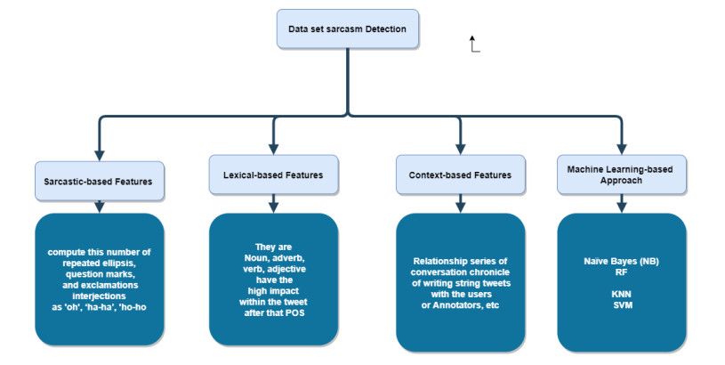
Sarcasm means the opposite of what you desire to express, particularly to insult a person. Sarcasm detection in social networks SNs such as Twitter is a significant task as it has assisted in studying tweets using NLP. Many existing study-related methods have always focused only on the content-based on features in sarcastic words, leaving out the lexical-based features and context-based features knowledge in isolation. This shows a loss of the semantics of terms in a sarcastic expression. This study proposes an improved model to detect sarcasm from SNs. We used three feature set engineering: context-based on features set, Sarcastic based on features, and lexical based on features. Two Novel Algorithms for an effective model to detect sarcasm are divided into two stages. The first used two algorithms one with preprocessing, and the second algorithm with feature sets. To deal with data from SNs. We applied various supervised machine learning (ML) such as k-nearest neighbor classifier (KNN), na?ve Bayes (NB), support vector machine (SVM), and Random Forest (RF) classifiers with TF-IDF feature extraction representation data. To model evaluation metrics, evaluate sarcasm detection model performance in precision, accuracy, recall, and F1 score by 100%. We achieved higher results in Lexical features with KNN 89.19 % accuracy campers to other classifiers. Combining two feature sets (Sarcastic and Lexical) has shown slight improvement with the same classifier KNN; we achieved 90.00% accuracy. When combining three feature sets (Sarcastic, Lexical, and context), the accuracy is shown slight improvement. Also, the same classifier we achieved is a 90.51% KNN classifier. We perform the model differently to see the effect of three feature sets through the experiment individual, combining two feature sets and gradually combining three feature sets. When combining all features set together, achieve the best accuracy with the KNN classifier.

| [1] |
Pawar N, Bhingarkar S (2020) Machine Learning based Sarcasm Detection on Twitter Data. 2020 5th International Conference on Communication and Electronics Systems (ICCES), 957‒961. https://doi.org/10.1109/ICCES48766.2020.9137924 doi: 10.1109/ICCES48766.2020.9137924

|
| [2] |
Suhaimin MSM, Hijazi MHA, Alfred R, et al. (2017) Natural language processing based features for sarcasm detection: An investigation using bilingual social media texts. 2017 8th International Conference on Information Technology (ICIT), 703‒709. https://doi.org/10.1109/ICITECH.2017.8079931 doi: 10.1109/ICITECH.2017.8079931
|
| [3] |
Bharti SK, Babu KS, and Raman R (2017) Context-based Sarcasm Detection in Hindi Tweets. 2017 9th Int. Conf. Adv. Pattern Recognition, ICAPR, 1–6. https://doi.org/10.1109/ICAPR.2017.8593198 doi: 10.1109/ICAPR.2017.8593198
|
| [4] | Zhang M, Zhang Y, Fu G (2016) Tweet sarcasm detection using deep neural network. COLING 2016 - 26th Int. Conf. Comput. Linguist. Tech. Pap., 2449–2460. |
| [5] |
Athira MR, Chithra C, Anil G, et al. (2020) Sentiment Analysis - Sarcasm Detection in Twitter. Journal of Computer Engineering (IOSR-JCE) 22: 42–46. https://doi.org/10.9790/0661-2204024246 doi: 10.9790/0661-2204024246
|
| [6] |
Prasad AG, Sanjana S, Bhat SM, and B. S. Harish (2017) Sentiment analysis for sarcasm detection on streaming short text data. 2017 2nd International Conference on Knowledge Engineering and Applications (ICKEA), 1‒5. https://doi.org/10.1109/ICKEA.2017.8169892 doi: 10.1109/ICKEA.2017.8169892
|
| [7] | Bindra KK, Prof A, Gupta A (2016) Tweet Sarcasm : Mechanism of Sarcasm Detection in Twitter. International Journal of Computer Science and Information Technologies 7: 215–217. |
| [8] |
Bharti SK, Vachha B, Pradhan RK, et al. (2016) Sarcastic sentiment detection in tweets streamed in real-time: a big data approach. Digit Commun Netw 2: 108–121. https://doi.org/10.1016/j.dcan.2016.06.002 doi: 10.1016/j.dcan.2016.06.002
|
| [9] |
Sarsam SM, Al-Samarraie H, Alzahrani AI, et al. (2020) Sarcasm detection using machine learning algorithms in Twitter: A systematic review. Int J Market Res 62: 578–598. https://doi.org/10.1177/1470785320921779 doi: 10.1177/1470785320921779
|
| [10] |
Bouazizi M, Ohtsuki T (2015) Sarcasm Detection in Twitter: "All Your Products Are Incredibly Amazing!!!" - Are They Really? 2015 IEEE Global Communications Conference (GLOBECOM), 1‒6. https://doi.org/10.1109/GLOCOM.2015.7417640 doi: 10.1109/GLOCOM.2015.7417640
|
| [11] |
Eke CI, Norman AA, Shuib L, et al. (2020) Sarcasm identification in textual data: systematic review, research challenges, and open directions. Artif Intell Rev 53: 4215–4258. https://doi.org/10.1007/s10462-019-09791-8 doi: 10.1007/s10462-019-09791-8
|
| [12] |
Saha S, Yadav J, Ranjan P (2017) Proposed Approach for Sarcasm Detection in Twitter. Indian J Sci Technol 10: 1–8. https://doi.org/10.17485/ijst/2017/v10i25/114443 doi: 10.17485/ijst/2017/v10i25/114443
|
| [13] | Sharma S, Chakraverty S (2018) SARCASM DETECTION IN ONLINE REVIEW TEXT. 1674–1679. |
| [14] |
Wen Z, Gui L, Wang Q, et al. (2022) Sememe knowledge and auxiliary information enhanced approach for sarcasm detection. Inf Process Manag 59: 102883. https://doi.org/10.1016/j.ipm.2022.102883 doi: 10.1016/j.ipm.2022.102883
|
| [15] |
Pawar N, Bhingarkar S (2020) Machine learning-based sarcasm detection on Twitter data. Proc 5th Int Conf Commun Electron Syst ICCES 2020, 957–961. https://doi.org/10.1109/ICCES48766.2020.9137924 doi: 10.1109/ICCES48766.2020.9137924
|
| [16] |
Halim Z, Waqar M, Tahir M (2020) A machine learning-based investigation utilizing the in-text features for the identification of dominant emotion in an email. Knowledge-Based Syst 208: 106443. https://doi.org/10.1016/j.knosys.2020.106443 doi: 10.1016/j.knosys.2020.106443
|
| [17] |
Jain T, Agrawal N, Goyal G, et al. (2017) Sarcasm detection of tweets: A comparative study. 2017 Tenth International Conference on Contemporary Computing (IC3), 1‒6, https://doi.org/10.1109/IC3.2017.8284317 doi: 10.1109/IC3.2017.8284317
|
| [18] | Biere S, Bhulai S, Analytics MB (2018) Hate Speech Detection Using Natural Language Processing Techniques. Vrije Univ. Amsterdam. |
| [19] | Konduri V, Padathula S, Pamu A, et al. (2020) Hate Speech Classification of social media posts using Text Analysis and Machine Learning. Oklahoma State University. |
| [20] |
Panda S, Kusum (2020) Detecting Twitter's Impact on COVID-19 Pandemic in India. Int J Innov Technol Explor Eng 9: 815–819. https://doi.org/10.35940/ijitee.H6718.069820 doi: 10.35940/ijitee.H6718.069820
|
| [21] |
Amer AYA, Siddiqui T (2020) Detection of Covid-19 Fake News text data using Random Forest and Decision tree Classifiers. International Journal of Computer Science and Information Security IJCSIS 18: 88–100. https://doi.org/10.5281/zenodo.4427204 doi: 10.5281/zenodo.4427204
|
| [22] | Shaalan K, Hassanien AE, Tolba F (2018) Intelligent Natural Language Processing: Trends and Applications. vol. 740, Springer. https://doi.org/10.1007/978-3-319-67056-0 |
| [23] |
Salloum SA, Al-Emran M, Monem AA, et al. (2018) Using text mining techniques for extracting information from research articles. Studies in Computational Intelligence 740: 373–397. https://doi.org/10.1007/978-3-319-67056-0_18 doi: 10.1007/978-3-319-67056-0_18
|
| [24] |
Kowsari K, Meimandi KJ, Heidarysafa M, et al. (2019) Text classification algorithms: A survey. Information 10: 150. https://doi.org/10.3390/info10040150 doi: 10.3390/info10040150
|
| [25] |
Nhlabano VV, Lutu PEN (2018) Impact of Text Preprocessing on the Performance of Sentiment Analysis Models for Social Media Data. 2018 Int Conf Adv Big Data, Comput Data Commun Syst icABCD, 1–6. https://doi.org/10.1109/ICABCD.2018.8465135 doi: 10.1109/ICABCD.2018.8465135
|
| [26] |
Dawei W, Alfred R, Obit JH, et al. (2021) A Literature Review on Text Classification and Sentiment Analysis Approaches. Lect Notes Electr Eng 724: 305–323. https://doi.org/10.1007/978-981-33-4069-5_26 doi: 10.1007/978-981-33-4069-5_26
|
| [27] |
Zhou Z, Guan H, Bhat MM, et al. (2019) Fake news detection via NLP is vulnerable to adversarial attacks. ICAART 2019 - Proc 11th Int Conf Agents Artif Intell 2: 794–800. https://doi.org/10.5220/0007566307940800 doi: 10.5220/0007566307940800
|
| [28] |
Mansour S (2018) Social media analysis of user's responses to terrorism using sentiment analysis and text mining. Procedia Comput Sci 140: 95–103. https://doi.org/10.1016/j.procs.2018.10.297 doi: 10.1016/j.procs.2018.10.297
|
| [29] |
Ahmad I, Yousaf M, Yousaf S, et al. (2020) Fake News Detection Using Machine Learning Ensemble Methods. Complexity 2020: 680–685. https://doi.org/10.1155/2020/8885861 doi: 10.1155/2020/8885861
|
| [30] |
Sharmin S, Zaman Z (2018) Spam detection in social media employing machine learning tool for text mining. Proc - 13th Int Conf Signal-Image Technol Internet-Based Syst SITIS 2017, 137–142. https://doi.org/10.1109/SITIS.2017.32 doi: 10.1109/SITIS.2017.32
|
| [31] |
Neeraja M, Prakash J (2016) Detecting Malicious Posts in Social Networks Using Text Analysis. International Journal of Science and Research (IJSR) 5: 345–347. https://doi.org/10.21275/v5i6.NOV164091 doi: 10.21275/v5i6.NOV164091
|
| [32] |
Hussain MG, Hasan MR, Rahman M, et al. (2020) Detection of Bangla Fake News using MNB and SVM Classifier. 2020 International Conference on Computing, Electronics & Communications Engineering (iCCECE). https://doi.org/10.1109/iCCECE49321.2020.9231167 doi: 10.1109/iCCECE49321.2020.9231167
|
| [33] |
Neha D, Vidyavathi BM (2015) A Survey on Applications of Data Mining using Clustering Techniques. International Journal of Computer Applications 126: 7–12. https://doi.org/10.5120/ijca2015905986 doi: 10.5120/ijca2015905986
|
| [34] |
Kaur R, Singh S (2016) FULL-LENGTH ARTICLE A survey of data mining and social network analysis based anomaly detection techniques. Egypt Informatics J 17: 199–216. https://doi.org/10.1016/j.eij.2015.11.004 doi: 10.1016/j.eij.2015.11.004
|
| [35] |
Sharath KA, Singh S (2013) Detection of user cluster with suspicious activity in online social networking sites. Proc - 2nd Int Conf Adv Comput Netw Secur ADCONS 2013, 220–225. https://doi.org/10.1109/ADCONS.2013.17 doi: 10.1109/ADCONS.2013.17
|
| [36] |
Al Mansoori S, Almansoori A, Alshamsi M, et al. (2020) Suspicious Activity Detection of Twitter and Facebook using Sentimental Analysis. TEM JOURNAL - Technology, Education, Management, Informatics TEM J 9: 1313–1319. https://doi.org/10.18421/TEM94-01 doi: 10.18421/TEM94-01
|
| [37] |
Rajeswari K, Shanthibala P (2018) SARCASM DETECTION USING MACHINE LEARNING TECHNIQUES. Int J Recent Sci Res 9: 26368–26372. http://dx.doi.org/10.24327/ijrsr.2018.0904.2046 doi: 10.24327/ijrsr.2018.0904.2046
|
| [38] |
Chen J, Yan S, Wong KC (2018) Verbal aggression detection on Twitter comment : convolutional neural network for short-text sentiment analysis. Neural Comput Appl 32: 10809‒10818. https://doi.org/10.1007/s00521-018-3442-0 doi: 10.1007/s00521-018-3442-0
|
| [39] |
Li Y, Li T (2013) Deriving market intelligence from microblogs. Decis Support Syst 55: 206–217. https://doi.org/10.1016/j.dss.2013.01.023 doi: 10.1016/j.dss.2013.01.023
|
| [40] |
Kharde VA, Sonawane SS (2016) Sentiment Analysis of Twitter Data: A Survey of Techniques. International Journal of Computer Applications 139: 5–15. https://doi.org/10.5120/ijca2016908625 doi: 10.5120/ijca2016908625
|
| [41] |
Joshi S, Deshpande D (2018) Twitter Sentiment Analysis System. International Journal of Computer Applications 180: 35–39. https://doi.org/10.5120/ijca2018917319 doi: 10.5120/ijca2018917319
|
| [42] |
Rui H, Liu Y, Whinston A (2013) Whose and what chatter matters? The effect of tweets on movie sales. Decis Support Syst 55: 863–870. https://doi.org/10.1016/j.dss.2012.12.022 doi: 10.1016/j.dss.2012.12.022
|
| [43] |
Ghosh D, Guo W, Muresan S (2015) Sarcastic or not: Word embeddings to predict the literal or sarcastic meaning of words. Conf Proc - EMNLP 2015 Conf Empir Methods Nat Lang Process, 1003–1012. https://doi.org/10.18653/v1/D15-1116 doi: 10.18653/v1/D15-1116
|
| [44] | Khodak M, Saunshi N, Vodrahalli K (2018) A large self-annotated corpus for sarcasm. Proceedings of the Eleventh International Conference on Language Resources and Evaluation (LREC 2018). |
| [45] |
Rahman AU, Halim Z (2022) Identifying dominant emotional state using handwriting and drawing samples by fusing features. Appl Intell 2022: 1‒17. https://doi.org/10.1007/s10489-022-03552-x doi: 10.1007/s10489-022-03552-x
|
| [46] |
Halim Z, Ali O, Khan MG (2021) On the Efficient Representation of Datasets as Graphs to Mine Maximal Frequent Itemsets. IEEE T Knowl Data Eng 33: 1674–1691. https://doi.org/10.1109/TKDE.2019.2945573 doi: 10.1109/TKDE.2019.2945573
|
| [47] |
Savini E, Caragea C (2022) Intermediate-Task Transfer Learning with BERT for Sarcasm Detection. Mathematics 10: 844. https://doi.org/10.3390/math10050844. doi: 10.3390/math10050844
|
| [48] |
Halim Z, Rehan M (2020) On identification of driving-induced stress using electroencephalogram signals: A framework based on wearable safety-critical scheme and machine learning. Inf Fusion 53: 66–79. https://doi.org/10.1016/j.inffus.2019.06.006 doi: 10.1016/j.inffus.2019.06.006
|


Figures(7) / Tables(9)

Abdullah Yahya Abdullah Amer, Tamanna Siddiqu. A novel algorithm for sarcasm detection using supervised machine learning approach[J]. AIMS Electronics and Electrical Engineering, 2022, 6(4): 345-369. doi: 10.3934/electreng.2022021


 DownLoad: