| Specie | Stand number | Area (ha) |
| Araucaria angustifolia | 32 | 482 |
| hybrid pine | 45 | 770 |
| Pinus taeda | 85 | 1.804 |
| Total | 162 | 3.056 |


Accurate abdomen tissues segmentation is one of the crucial tasks in radiation therapy planning of related diseases. However, abdomen tissues segmentation (liver, kidney) is difficult because the low contrast between abdomen tissues and their surrounding organs. In this paper, an attention-based deep learning method for automated abdomen tissues segmentation is proposed. In our method, image cropping is first applied to the original images. U-net model with attention mechanism is then constructed to obtain the initial abdomen tissues. Finally, level set evolution which consists of three energy terms is used for optimize the initial abdomen segmentation. The proposed model is evaluated across 470 subsets. For liver segmentation, the mean dice are 96.2 and 95.1% for the FLARE21 datasets and the LiTS datasets, respectively. For kidney segmentation, the mean dice are 96.6 and 95.7% for the FLARE21 datasets and the LiTS datasets, respectively. Experimental evaluation exhibits that the proposed method can obtain better segmentation results than other methods.
Citation: Zhaoxuan Gong, Jing Song, Wei Guo, Ronghui Ju, Dazhe Zhao, Wenjun Tan, Wei Zhou, Guodong Zhang. Abdomen tissues segmentation from computed tomography images using deep learning and level set methods[J]. Mathematical Biosciences and Engineering, 2022, 19(12): 14074-14085. doi: 10.3934/mbe.2022655
| [1] | Feng Guo, Haiyu Xu, Peng Xu, Zhiwei Guo . Design of a reinforcement learning-based intelligent car transfer planning system for parking lots. Mathematical Biosciences and Engineering, 2024, 21(1): 1058-1081. doi: 10.3934/mbe.2024044 |
| [2] | Wenyang Gan, Lixia Su, Zhenzhong Chu . A PSO-enhanced Gauss pseudospectral method to solve trajectory planning for autonomous underwater vehicles. Mathematical Biosciences and Engineering, 2023, 20(7): 11713-11731. doi: 10.3934/mbe.2023521 |
| [3] | Na Li, Peng Luo, Chunyang Li, Yanyan Hong, Mingjun Zhang, Zhendong Chen . Analysis of related factors of radiation pneumonia caused by precise radiotherapy of esophageal cancer based on random forest algorithm. Mathematical Biosciences and Engineering, 2021, 18(4): 4477-4490. doi: 10.3934/mbe.2021227 |
| [4] | Daiver Cardona-Salgado, Doris Elena Campo-Duarte, Lilian Sofia Sepulveda-Salcedo, Olga Vasilieva, Mikhail Svinin . Optimal release programs for dengue prevention using Aedes aegypti mosquitoes transinfected with wMel or wMelPop Wolbachia strains. Mathematical Biosciences and Engineering, 2021, 18(3): 2952-2990. doi: 10.3934/mbe.2021149 |
| [5] | Baoye Song, Shumin Tang, Yao Li . A new path planning strategy integrating improved ACO and DWA algorithms for mobile robots in dynamic environments. Mathematical Biosciences and Engineering, 2024, 21(2): 2189-2211. doi: 10.3934/mbe.2024096 |
| [6] | Zhen Zhou, Chenchen Geng, Buhu Qi, Aiwen Meng, Jinzhuang Xiao . Research and experiment on global path planning for indoor AGV via improved ACO and fuzzy DWA. Mathematical Biosciences and Engineering, 2023, 20(11): 19152-19173. doi: 10.3934/mbe.2023846 |
| [7] | Poonkuzhali Sugumaran, Vinodhkumar Sukumaran . Recommendations to improve dead stock management in garment industry using data analytics. Mathematical Biosciences and Engineering, 2019, 16(6): 8121-8133. doi: 10.3934/mbe.2019409 |
| [8] | Qiuyi Su, Jianhong Wu . Impact of variability of reproductive ageing and rate on childhood infectious disease prevention and control: insights from stage-structured population models. Mathematical Biosciences and Engineering, 2020, 17(6): 7671-7691. doi: 10.3934/mbe.2020390 |
| [9] | Gaozhong Sun, Tongwei Zhao . Lung adenocarcinoma pathology stages related gene identification. Mathematical Biosciences and Engineering, 2020, 17(1): 737-746. doi: 10.3934/mbe.2020038 |
| [10] | N Arunkumar, B Nagaraj, M Ruth Keziah . EpilepIndex: A novel feature engineering tool to detect epilepsy using EEG signals. Mathematical Biosciences and Engineering, 2023, 20(12): 21670-21691. doi: 10.3934/mbe.2023959 |
Accurate abdomen tissues segmentation is one of the crucial tasks in radiation therapy planning of related diseases. However, abdomen tissues segmentation (liver, kidney) is difficult because the low contrast between abdomen tissues and their surrounding organs. In this paper, an attention-based deep learning method for automated abdomen tissues segmentation is proposed. In our method, image cropping is first applied to the original images. U-net model with attention mechanism is then constructed to obtain the initial abdomen tissues. Finally, level set evolution which consists of three energy terms is used for optimize the initial abdomen segmentation. The proposed model is evaluated across 470 subsets. For liver segmentation, the mean dice are 96.2 and 95.1% for the FLARE21 datasets and the LiTS datasets, respectively. For kidney segmentation, the mean dice are 96.6 and 95.7% for the FLARE21 datasets and the LiTS datasets, respectively. Experimental evaluation exhibits that the proposed method can obtain better segmentation results than other methods.
Forests and forest industries play an important role in economic and social development in the northeast of Argentina, especially in the provinces of Misiones and Corrientes. Efficient planning is essential at all levels to achieve a competitive forestry industry. Forest-management planning could be addressed at various temporal scales. Strategic planning is associated with extended temporal horizons whereas tactical planning focuses on shorter periods of time and typically encompass further spatial requirements (Bellavenutte, et al. [1]). According to Borges et al. [2] strategic or long-term management planning typically encompasses temporal horizons extending over more than 10 years so that forest economic and biological processes may be adequately known. Furthermore, the same authors emphasize that management planning is one of the most important problems that foresters must face.
Strategic planning is particularly important as it seeks to regulate forest production in the long-term and increase forest income to ensure sectorial competitiveness (Andersson [3]; Broz [4]). The multidimensionality of the system makes this process complex, and the aid of mathematical models is essential (Broz [5]). In this sense, linear programming is a robust tool to solve this type of problem. The first models applied to forest sciences were developed in the 60s by Gilmore and Gomory [6], Curtis [7] and Pnevmaticos and Mann [8]. However, the approach of Johnson and Scheurman [9] defines the bases of strategic planning based on an alternative formulation of the linear programming harvest scheduling problem which they called Model type Ⅰ and Ⅱ. Afterwards, Barros and Weintraub [10] developed a planning model for vertical industries demonstrating the need for wood production zones to be divided into areas with uniform characteristics. On the other hand, Gassmann [11] relies on stochastic optimization techniques to find the income levels that maximize the harvest in a finite horizon and under risky conditions. Thus far, different approaches and applications have been published. Due to computational limitations, the first models were relatively minor, but nowadays it is possible to tackle large problems using standard computers.
Currently there are numerous developments applied to different contexts in the forestry sector, for example strategic, tactic and operative planning; transport; log cutting; sawmill process; among others (Broz, [5], Bellavenutte, et al. [12]). In this sense, Banhara et al. [13] seeks a mixed integer linear programming model with minimization of target deviations to improve operational planning techniques for eucalyptus harvest. On the other hand, Da Silva [14] studied models of use divided into blocks and parcels to minimize the costs of use and maintenance of the forest road network through Mixed Whole Linear Programming (PLIM). Pereira [15] applies an optimized tactical planning for the Eucalyptus spp forest harvest considering annual harvest blocks. Viana Céspedes [16] proposes a combinatorial optimization model based on the problem of the multiple traveling salesperson with multiple deposits as a tool to support harvest scheduling and equipment allocation for contractor companies. Paradis et al. [17] presented a two-level formulation, based on a classical wood supply optimization model, which explicitly anticipates the consumption of industrial fibers. Troncoso et al. [18] presented a model of the supply chain of a vertically integrated firm. The goal is to determine which stand to cut and when and where to send each of its products. In addition, the literature presents multiple objective models, in which the decision-maker must plan a compromising situation among several defined aspects. Among these, we can cite the works of Broz [5], Silva et al. [19], Diaz-Balteiro et al. [20], Giménez et al. [21], Bellavenutte et al. [12] and others.
The mathematical optimization applications have been carried out since the 60s (Bettinger and Chung [22]). Furthermore, the applications are carried out in different areas of the forest value chain, from primary production (silviculture, harvesting, transport and others) to transformation (cutting pattern, optimization process, drying and others). In addition, we conclude that different approaches to mathematical optimization are presented, such as deterministic, stochastic, mono-objective and multi-objective models. Despite the large amount of information on the mathematical models applied to the forestry sector, by adopting these tools, the company must be cautious. In this sense, different models and constraints must be evaluated to define which of them meets expectations set by the organization.
In this work, we evaluated four mathematical model variants, based on Johnson and Scheurman's [9] model, were evaluated. The first mathematical model seeks to minimize the difference between the extreme values of production; the second model seeks to minimize the absolute deviations of log productions between consecutive years; the third model seeks to maximize the net present value (NPV) and balancing log production between consecutive years; and finally, the fourth model seeks to maximize the NPV and balancing log production based on the first year of the planning horizon. Besides, we seek to plan the change of cultivated species with the objective of achieving a monospecific forest heritage. The objective of this work was to evaluate different mathematical models (objective functions and constraints) as forest planning tools, both in volume regulation and in cultivated species change policy. In addition, it sought to show the effect of flexibilization of the harvest age on the interannual production of logs.
The authors compare different mathematical models for forest regulation, both objective functions and constraints. In this sense, we seek to highlight the advantages and disadvantages of each approach in such a way that the decision maker adopts a model according to their organization objectives. We pretend demonstrate the effect of harvest age flexibilization in production regulation and the impact of resulting management regimes on forest value. Finally, we intend to show that the models and the regulating production allow defining a policy of species change without compromising production volumes.
The paper is structured as follows. Section 2 presents the methodology that describes the study area, current forest management and its limitations, as well as another management proposal. Then, the main features of the model and a description of the application is presented. Section 3 presents the results of applying the models and section 4 summarizes the main conclusions derived from this research.
The study area belongs to a forest heritage located in the north of the province of Misiones. The land use is a forest plantation with Pinus taeda (Pt), Pinus elliottii var. elliottii x Pinus caribaea var. hondurensis or hybrid pine (Hp) and Araucaria angustifolia (Aa) belonging to a forest heritage located in the north of the province of Misiones. This case corresponds to a total of 162 stands representing an area of 3056 ha, with an age range from 1 to 36 years. In table 1 the number of stand and area for each species is shown.
| Specie | Stand number | Area (ha) |
| Araucaria angustifolia | 32 | 482 |
| hybrid pine | 45 | 770 |
| Pinus taeda | 85 | 1.804 |
| Total | 162 | 3.056 |
 DownLoad:
CSV
DownLoad:
CSV
The forest has a traditional forest management scheme which is 3-4 thinnings and rotation age older than 18 years (Pt and Hp) and 25 years (Aa) to produce large logs. In Table 2, intervention type, intensity and opportunity of the silvicultural action of the company is detailed. In management activities, the following costs were considered: planting and maintenance for 3 years: 951.51 USD/ha; pruning 1: 114.59 USD/ha; pruning 2: 117.1 USD/ha; pruning 3: 147.82 USD/ha; administrative costs: 50 USD/ha/year (COIFORM [23]).
| Species | Intervention | Tree removed (%) | Age (years) |
| Araucaria angustifolia - Initial density 2,222 trees/ha - 3 pruning | 1° thinning | 50 | 8 |
| 2° thinning | 40 | 11 | |
| 3° thinning | 40 | 15 | |
| 4° thinning | 40 | 20 | |
| Clear-cutting | 100 | 25 | |
| Pinus taeda - Initial density 1,667 trees/ha - 2 pruning |
1° thinning | 55 | 6 |
| 2° thinning | 40 | 9 | |
| 3° thinning | 40 | 13 | |
| Clear-cutting | 100 | 18 | |
| Hybrid pine - Initial density 1,333 trees/ha - 2 pruning |
1° thinning | 50 | 7 |
| 2° thinning | 40 | 10 | |
| 3° thinning | 40 | 14 | |
| Clear-cutting | 100 | 18 |
DownLoad:
CSV
The current forest management scheme is very rigid, and this does not allow an adequate balance of interannual log production. This means that there are years with high log production and years of low production. In this case, a more flexible clear-cutting age was proposed. Thus, the clear-cutting age is relaxed by ±1 (that is, 3 clear-cutting age options) and the following clear-cutting age is relaxed by ±2 years (5 clear-cutting age options).
In this sense, the factory demands logs with a maximum small end diameter1 (SED) of 24 cm, but current forest management points to produce thick logs. The ones with a SED greater than 24 cm represent 48% of the total volume. In addition, pulp logs represent 10%; but logs with a maximum SED of 24 cm represent less than 42% of the total volume. In this case, it is proposed to eliminate a thinning operation for each species.
1 The small end diameter or SED is the smallest diameter of a log and it is given by its conicity.
Currently, Pt and Aa represent 75% of the forest. Pt have more conicity and a higher yield (33 m3/ha/year) whereas Aa have less conicity and a low yield (24 m3/ha/year). On the other hand, the Hp has a good yield (34 m3/ha/year), less conicity and fine branches, which allows good pruning and higher industrial performance. Furthermore, Ph has physical and mechanical properties equal to, or greater than, Aa and Pt. For these reasons, a new management policy, to replace Pt and Aa stands by Ph was proposed.
Currently, the company carries out the planning process empirically, using a spreadsheet. In this situation, we proposed the use of mathematical optimization models as decision support tools. In addition, we demonstrated the flexibility of the tools in the face of changes in forest management policy. These models are evaluated in a planning horizon of 50 years, from 2022 to 2071, and for the calculation of profitability, a discount rate of 10% is used.
Table 3 shows log characteristics taken from the forest according to the species, SED, length and market prices put at the sawmill subtracting average costs of thinning, harvest and transport (COIFORM, [23]). In other words, these prices are named standing timber prices. These data are used to simulate forest management regimens.
| Specie | SED (cm) | Log length (ft) | Price (USD/t) | Id reference |
| Pinus taeda | 35–99 | 14 | 13, 88 | Pt35_99 |
| Pinus taeda | 29–35 | 14 | 8, 23 | Pt29_35 |
| Pinus taeda | 25–29 | 14 | 3, 7 | Pt25_29 |
| Pinus taeda | 18–25 | 10 | 2, 37 | Pt18_25 |
| Pinus taeda | 14–18 | 10 | 1, 99 | Pt14_18 |
| Pinus taeda | < 14 | 8 | 1, 21 | PtPulp |
| Hibrid pine | 35–99 | 14 | 13, 88 | Hp35_99 |
| Hibrid pine | 29–35 | 14 | 8, 23 | Hp29_35 |
| Hibrid pine | 25–29 | 14 | 3, 7 | Hp25_29 |
| Hibrid pine | 18–25 | 10 | 2, 37 | Hp18_25 |
| Hibrid pine | 14–18 | 10 | 1, 99 | Hp14_18 |
| Hibrid pine | < 14 | 8 | 1, 21 | HpPulp |
| Araucaria angustifolia | 35–99 | 14 | 36, 3 | Aa35_99 |
| Araucaria angustifolia | 29–35 | 14 | 20, 68 | Aa29_35 |
| Araucaria angustifolia | 25–29 | 14 | 20, 68 | Aa25_29 |
| Araucaria angustifolia | 18–25 | 10 | 9, 33 | Aa18_25 |
| Araucaria angustifolia | 14–18 | 10 | 5, 66 | Aa14_18 |
| Araucaria angustifolia | < 14 | 8 | 1, 21 | AaPulp |
DownLoad:
CSV
In Table 4, everything related to the model is listed, such as, index, variables and parameters, with a short description and corresponding units. Every model considers a 50-year planning horizon divided into 50 periods of 1-year each. The objectives of model 1 (Eqs 1–4) and 2 (Eqs 5–8) are intended to stabilize the global production of the forest. On the other hand, model 3 (Eqs 9–12) and 4 (Eqs 13–16) we seek to maximize NPV, considering costs and revenues. All management regimes consider not only current stand situation, but future cycles too.
| Description | |
| Index | |
| i | Stands, i = 1, …, M |
| j | Silvicultural prescriptions, j = 1, …, N |
| t | Period, p = 1, …, H |
| Variable | |
| Xij | The area of stand i to be managed according to prescription j. |
| MinMax | The lowest volume from maximum production volume in the planning horizont. |
| MaxMin | The highest volume of the minimum possible production in the planning horizon. |
| VOLDEV | The absolute volume deviation (m3) in consecutive years. |
| MinDIF | Dependent variable (m3) representing the difference between the extreme maximum and minimum volumes. |
| MinDEV | Dependent variable (m3) representing the minimum absolute deviations of log productions among consecutive years. |
| MaxNPV | Dependent variable (USD) representing the maximum NPV. |
| Parameter | |
| VOLijt | Volume (m3) obtained from stand i at period t according to prescription j, determined from the simulation process. |
| Ai | Area of stand i (ha). |
| NPVij | Net present value (USD) from stand i managed whit prescription j. |
| u | Production relaxation factor (<1) between t. |
DownLoad:
CSV
Model M1: This model seeks to minimize the difference between the extreme values of production (Eq 1) avoiding harvesting a surface larger than that available in each stand i.e., maximum area of each stand (Eq 2). Additional constraints (Eq 3) are required to minimize the difference between the maximum and minimum annual log production. Here, the lowest volume from maximum production volume and the highest volume of the minimum production volume in the planning horizon is obtained and it will be minimized in the objective function. Finally, the type of variable must be defined (Eq 4) to ensure that the harvest area was positive.
| MinDIF=Min(MinMax−MaxMin) | (1) |
| N∑j=1Xij≤Ai;∀i | (2) |
| M∑i=1N∑j=1(VOLijtXij)≤MinMax;∀tM∑i=1N∑j=1(VOLijtXij)≥MaxMin;∀t | (3) |
| Xij≥0;∀i,j | (4) |
Model M2: This model seeks to minimize the absolute deviations of log productions between consecutive years (Eq 5) given the maximum area of each stand (Eq 6), similar to Eq 2 of the model M1. Additional constraints (Eq 7) seek to compute the absolute deviations of log harvest between consecutive years. In this case, absolute volume deviation in consecutive years is supposed to minimize in objective function. As in the previous model, the type of the variables must be established (Eq 8).
| MinDEV=VOLDEV | (5) |
| N∑j=1Xij≤Ai;∀i | (6) |
| M∑i=1N∑j=1(VOLijtXij)−M∑i=1N∑j=1(VOLijt−1Xij)<VOLDEV;∀t>1M∑i=1N∑j=1(VOLijt−1Xij)−M∑i=1N∑j=1(VOLijtXij)<VOLDEV;∀t>1 | (7) |
| Xij≥0;∀i,j | (8) |
Model M3: This model seeks to maximize NPV (Eq 9) given the maximum area of each stand (Eq 10). Here, NPV depends on the discount rate chosen which is uploaded on software used to solve these models. In this case, balancing log production between consecutive years was defined, i.e., between t and t-1 (Eq 11). In other words, these constraints seek to establish a balance to avoid oscillations in of logs supply in consecutive periods of planning horizon. In addition, a parameter u is defined to relax the constraint to avoid infeasible solutions. As in the previous model, the type of the variables must be established (Eq 12).
| MaxNPV=M∑i=1N∑j=1NPVij×Xij | (9) |
| N∑j=1Xij≤Ai,∀i | (10) |
| M∑i=1N∑j=1Volijt×Xij≥(1−u)×M∑i=1N∑j=1Volij(t−1)×Xij;∀tM∑i=1N∑j=1Volijt×Xij≤(1+u)×M∑i=1N∑j=1Volij(t−1)×Xij;∀t | (11) |
| Xij≥0,∀i,j | (12) |
Model M4: This model seeks to maximize NPV (Eq 13) given the maximum area of each stand (Eq 14). Unlike model M3, the aim here is to balance log production based on the first year (t = 1) of the planning horizon (Eq 15). As in the preceding model, a parameter u is defined to relax the constraint to avoid infeasible solutions and the type of the variables must be established (Eq 16). Hence, the difference between models M3 and M4 lies in Eqs 11 and 15 respectively. In Eq 11 the production balance is made between consecutive periods, while in Eq 15 the balance is made between each period and the first period of the planning horizon.
| MaxNPV=M∑i=1N∑j=1NPVij×Xij | (13) |
| N∑j=1Xij≤Ai,∀i | (14) |
| M∑i=1N∑j=1Volijt×Xij≥(1−u)×M∑i=1N∑j=1Volij(t=1)×Xij;∀tM∑i=1N∑j=1Volijt×Xij≤(1+u)×M∑i=1N∑j=1Volij(t=1)×Xij;∀t | (15) |
| Xij≥0,∀i,j | (16) |
These models were implemented in Optimber-LP software for strategic forest planning and developed by Optimber Company. For the simulation of forest management regimes, Optimber-LP uses the SisPTaeda simulation package, developed by Empresa Brasileira de Pesquisa Agropecuária (EMBRAPA) for the projection of forest growth. On the other hand, to solve mathematical optimizations models, Optimber-LP uses LINGO, a software developed by Lindo System Inc. The data required to model are stand, species, age, site index, area, year of planting, initial density, basal area, pruning height and number of thinnings carried out. All data are provided by the company through forest inventories for commercial purposes. The implementation was carried out on a computer with Intel Core i5-2310M, CPU @ 2.10 GHz, 8 GB of RAM and 64-bit OS.
To evaluate the models and the effect of relaxation, diverse scenarios are proposed which are based on the combination of the type of model and the clear-cut age relaxing (CAR). Table 5 describes each one.
| Model M1 | Without CAR | We seeks to minimize the difference between the extreme values of production but without clear-cut age relaxing. |
| Model M2 | Without CAR | We seeks to minimize the absolute deviations of log productions between consecutive years but without clear-cut age relaxing. |
| Model M1 | CAR ± 1 year | We seeks to minimize the difference between the extreme values of production with a clear-cut age relaxing of ±1 year, i.e., with three harvest age options. |
| Model M2 | CAR ± 1 year | We seeks to minimize the absolute deviations of log productions between consecutive years with a clear-cut age relaxing of ±1 year, i.e., with three harvest age options. |
| Model M1 | CAR ± 2 year | We seeks to minimize the difference between the extreme values of production with a clear-cut age relaxing of ±2 year, i.e., with five harvest age options. |
| Model M2 | CAR ± 2 year | We seeks to minimize the absolute deviations of log productions between consecutive years with a clear-cut age relaxing of ±2 year, i.e., with five harvest age options. |
| Model M3 | CAR ± 1 year | We seeks to maximize NPV and balancing log production between consecutive years with a clear-cut age relaxing of ±1 year, i.e., with three harvest age options. |
| Model M4 | CAR ± 1 year | We seeks to maximize NPV and balancing log production based on the first year with a clear-cut age relaxing of ±1 year, i.e., with three harvest age options. |
| Model M3 | CAR ± 2 year | We seeks to maximize NPV and balancing log production between consecutive years with a clear-cut age relaxing of ±2 year, i.e., with five harvest age options. |
| Model M4 | CAR ± 2 year | We seeks to maximize NPV and balancing log production based on the first year with a clear-cut age relaxing of ±2 year, i.e., with five harvest age options. |
DownLoad:
CSV
In Table 6, the statistics of the proposed scenarios, namely, number of variables, number of constraints, computation time, number of iterations and nonzeros elements are shown for all models and CAR. In all cases, the models do not exceed 114,000 variables and these have a reasonably low computation time, less to 88 seconds.
| N° variables | N° constraints | Time resolution (s) | N° iterations | Nonzeros | ||
| Model M1 | Without CAR | 31,122 | 44,391 | 1 | 0 | 121,541 |
| Model M2 | Without CAR | 31,121 | 44,389 | 1 | 0 | 121,634 |
| Model M1 | CAR ± 1 year | 42,530 | 44,391 | 13 | 2,821 | 991,334 |
| Model M2 | CAR ± 1 year | 42,529 | 44,389 | 13 | 3,056 | 991,427 |
| Model M1 | CAR ± 2 year | 113,329 | 44,391 | 79 | 1,803 | 6,440,444 |
| Model M2 | CAR ± 2 year | 113,328 | 44,389 | 88 | 2,821 | 6,440,537 |
| Model M3 | CAR ± 1 year | 42,528 | 44,389 | 13 | 927 | 1,004,698 |
| Model M4 | CAR ± 1 year | 42,528 | 44,389 | 13 | 841 | 1,004,698 |
| Model M3 | CAR ± 2 year | 113,327 | 44,389 | 76 | 917 | 6,524,607 |
| Model M4 | CAR ± 2 year | 113,327 | 44,389 | 74 | 917 | 6,524,607 |
DownLoad:
CSV
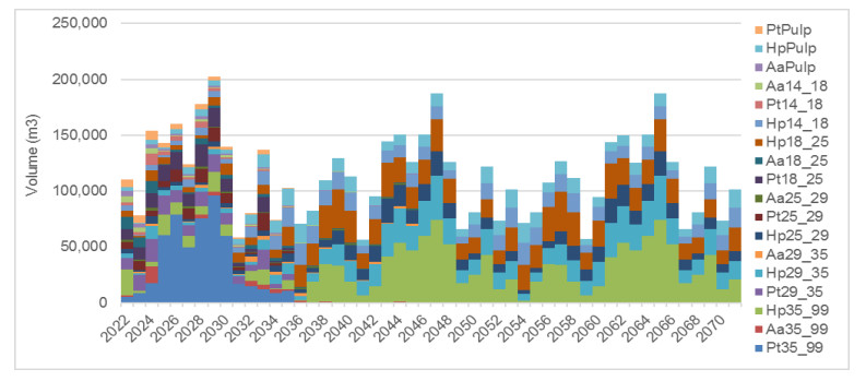
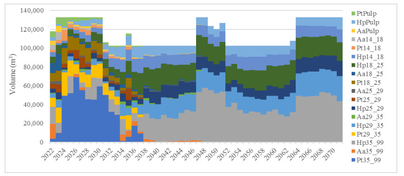
In Figure 1 shows the volumes obtained for each product (see Table 3, Id reference) without clear-cutting age relaxing in a 50-year forestry planning horizon. In this case, a significant oscillation is observed in the log production, this is between 56,000 and 202,000 m3/year. According to Bettinger et al. [24] and Broz et al. [4], a stand-level decision is carried out and the main problem lies in the instability of log supply and a consequence is the purchase of logs. Besides, this scenario is unrealistic, especially in integrated companies, and some strategies must be established to avoid the year-on-year oscillation. Here, there is a strong variation of the area affected to plantation, thinning (1, 2, 3 and 4) and clear felling. This variation has a direct correlation with the volume of logs harvested. In this case, the minimum and maximum planting and harvesting area was 34 and 380 ha/year respectively since the harvested area is immediately reforested. On the other hand, thinning ranges between 0 and 381 ha per year. A coefficient of variation of 55% was observed in planting and harvesting area and 59% in thinning.
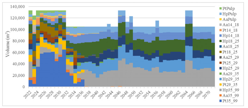
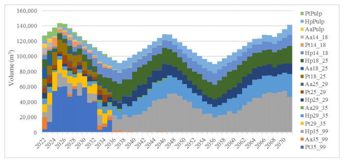
By applying model M1, the volume stabilized at 105,000 m3/year, with a maximum of 133,000 m3/year. At the beginning of the planning, the logs volume was higher because the forest was made up mostly by stands of adult stage trees (Figure 2). On the other hand, when model M2 is applied, the production of logs ranges between 94,000 and 140,000 m3/year, with an average of 114,000 m3/year. However, it presents an upward and downward inter-annual variation; this is because the regulation of production is carried out between consecutive years (Figure 3). Regarding the change of species, when planning in forest with model M1, at 25 years (2046) there is complete replacement of Pt and Aa stands by Hp, however, when model M2 is applied the replacement occurs in year 24 (2045). In this case, a moderate variation of the area affected to plantation, thinning (1, 2, 3 and 4) and clear felling is obtained, and it is similar for both models. The minimum and maximum planting and harvesting area was 103 and 240 ha/year respectively with 22% of coefficient of variation. Otherwise, the thinning ranges between 15 and 300 ha per year and coefficient of variation of 34%.
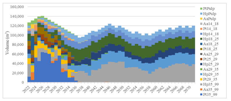
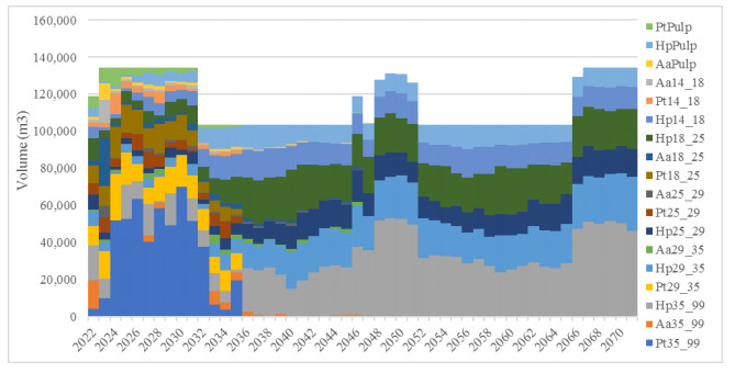
With model M1, the volume stabilizes at 105,000 m3/year. In this case, a very stable production is presented with an average production of 115,000 m3/year, a minimum of 112,000 m3/year and a maximum of 123,000 m3/year. This maximum volume occurs at the beginning of the planning horizon and, as mentioned, a high percentage of stands is due to adulthood (Figure 4). When using model M2, the average logs production is 113,000 m3/year, with a maximum of 126,000 m3/year, which occurs at the beginning of the planning horizon, and a minimum of 103,000 m3/year, which occurs at the end of the horizon. In this case, although production is stable, it is decreasing. Hence, it does not allow determining the regular forest volume (Figure 5). Regarding the change of species, when planning in forest with model M1, at 26 years (2047) there is complete replacement of Pt and Aa stands by Hp. However, when model M2 is applied the replacement occurs in year 22 (2043). Here, a moderate variation of the area affected to plantation, thinning (1, 2, 3 and 4) and clear felling is obtained, and it is similar for both models. In this case, the minimum and maximum planting and harvesting area was 89 and 265 ha/year respectively and 17% of coefficient of variation. On the other hand, the thinning ranges between 20 and 265 ha per year with 28% of coefficient of variation.
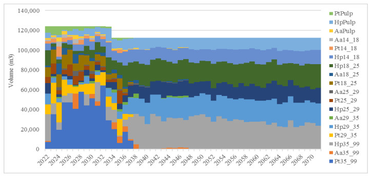
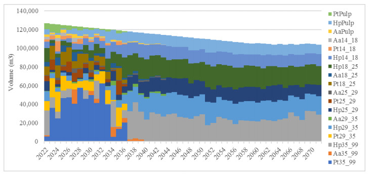
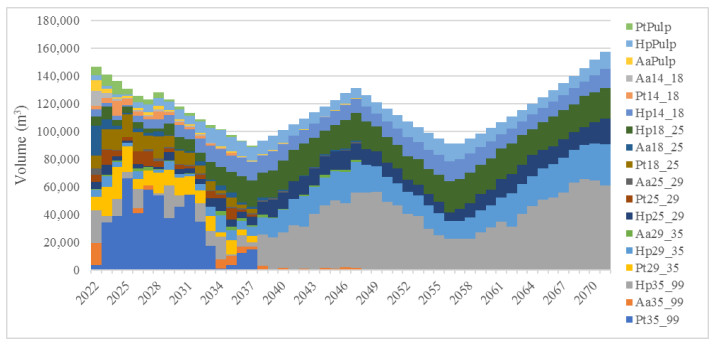
Figure 6 shows the volumes obtained for each product by applying model M3 and clear-cut age relaxing ±1 year is defined. At this point, we have observed a moderated oscillation in the log production with a minimum of 89,000 m3/, a maximum of 143,000 m3/year and an average of 115,000 m3/year; and USD 7,348,416 is the NPV obtained. In this case, we have observed an upward and downward inter-annual log production variation due to constraint 11 with the interannual regulation being carried out between consecutive years, i.e., t and t-1. On the other hand, when model M4 is applied, the production of logs ranges between 103,000 and 134,000 m3/year, with an average of 115,000 m3/year (Figure 7) and USD 7,449,453 is the NPV, 1.34% more than model M3. Here, the interannual production is more stable given that the minimum level of logs is defined based on the first year of the planning horizon, determined in constraint 15. Regarding the change of species, when planning a forest with model M3 and model M4, at 25 years (2046) there is complete replacement of Pt and Aa stands by Hp. As in the previous case, we have detected a moderate variation of the area affected to plantation, thinning and clear-cut and it is similar for both models. In this case, the minimum and maximum planting and harvesting area was 74 and 308 ha/year respectively with 31% of coefficient of variation. Otherwise, the thinning ranges between 15 and 300 ha per year and coefficient of variation of 39%.
In Figures 8 and 9 you can see the volumes obtained for each product by applying models M3 and M4 respectively, and clear-cut age relaxing ±2 year is defined. As in the preceding case, a moderated oscillation is observed in the log production where 89,000 m3/year is the minimum, 157,000 m3/year is the maximum and 115,000 m3/year is the average and USD 7.449.453 is the NPV obtained. The behavior of the volume produced is like that obtained when clear-cutting age relaxing is ±1 year. By applying model M4 the production of logs ranges between 102,000 and 133,000 m3/year, with an average of 115,000 m3/year (Figure 9) and USD 7.425.060 is the NPV, 1.42% more than model 3. In Model M4, the interannual production is quite stable given that the minimum level of logs is defined on the basis of the first year of the planning horizon. Regarding the change of species, when planning a forest with model M3 and model M4 and clear-cutting age relaxing is ±1 year, at 27 years (2047) there is complete replacement of Pt and Aa stands by Hp. Here, a moderate variation of the area affected to plantation, thinning and clear-cut is detected and it is similar for both models. In this case, the minimum and maximum planting and harvesting area was 85 and 317 ha/year respectively with 34% of coefficient of variation. For other part, the thinning ranges between 15 and 233 ha/year and coefficient of variation of 38%.
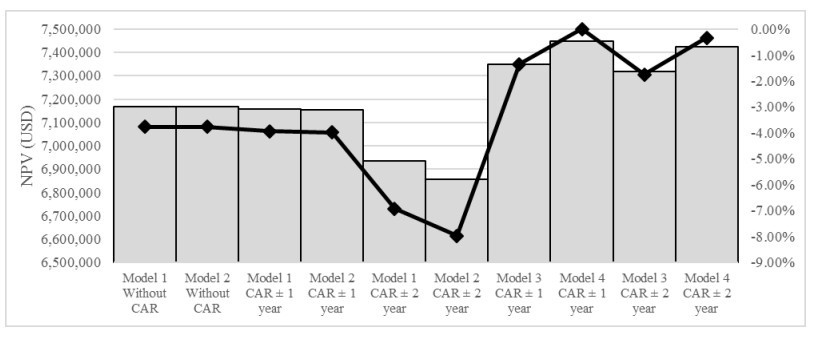
The economic performance of each combination between model and clear-cutting relaxing is presented in Figure 10. By optimized volume (models M1 and M2) without clear-cut age relaxing, model M1 and model M2 generated a NPV of USD 7,168,742 but, when clear-cutting was relaxing in ±1 year, the NPV of model M1 and model M2 was 0.18% and 0.23% less than scenario without clear-cut age relaxing. When clear-cutting was relaxing in ±2 year, the NPV of model M1 and model M2 was 3.29% and 4.38% less than scenario without clear-cutting age relaxing. On the other hand, when the NPV is optimized, the economic value is 1.04% higher than the scenarios in which the volume is optimized. Here, the model M4 and clear-cutting relaxing in ±1 year showed the largest NPV and the variation between these scenarios is less than 1.75%.
An overall analysis of the results shows large fluctuations in harvest volume when harvesting age is restricted. Similar results were obtained by Augustynczik et al. [25] and Augustynczik [26]. In order to stabilize logs production, better results are obtained when harvest age is relaxed in ±2 years because management prescriptions (options) are increased and, consequently, the mathematical model becomes more flexible as a result of increasing the feasible region (Winston and Goldberg, [27]). According to McDill [28] a large number of potential prescriptions for each management unit is essential to have a computer program which can simulate different prescriptions for each unit based on the attributes of the unit and to populate a database with parameters quantifying the inputs and outputs for each prescription for each management unit.
Furthermore, we demonstrate that model M1 presents better behavior than model M2 because it stabilizes production in the planning horizon. On the other hand, when we seek to maximize NPV, the stabilization of production only through a constraint. Results obtained with model M3 are similar to those of Broz et al. [4] and Vielma et al. [29]. Yet, the results obtained in model M4 are similar to Augustynczik [26], however, this author does not show volumes by products. The production balance constraint in the the first year of the planning horizon presents a better regulation of production than the constraint that regulates production between years. Models M2 and M3 present a narrow perspective problem since they compute volumes between consecutive years, which generates significant deviations in the planning horizon. In order to solve the narrow perspective problem of models M2 and M3, we recommend to establish a minimum and maximum volume limits based on an average harvest volume. In this sense, a minimum and maximum level must be established from the average harvest volume, relaxing ±2%, ±4%, ±6%, and so on until a feasible solution is found. Furthermore, the results improve if the harvest age is relaxed by ±2.
Relaxing the clear-cut age leads to a better balance in planting, thinning (1, 2, 3 and 4) and clear felling operations. However, no significant differences were found between ±1 and ±2 years, for the four models.
We show that rigid forest management scheme based on optimal harvesting at stand level generates problems in log supply to industries. In addition, the areas intervened for planting, thinning (1, 2, 3 and 4) and clear-cutting show large interannual variations. As a result, the allocation of resources varies significantly from year to year.
We presented four mathematical models to planning the forest production in a horizon of 50 years. Models M1 and M2 aim to stabilize production and Models M3 and M4 aim to maximize NPV. The four models presented different results according to their objectives and constraint. We found that when maximizing the economic benefit, the NPV is slightly higher, but it is not significant. In this sense, it is up to the planner to choose an economic or volumetric objective function according to the objectives planned by the organization.
The models succeeded in replacing the Aa and Pt stands with Hp at the time of clear felling. This, converting the forest heritage into monospecific. Although this is not something desirable from the environmental point of view, the forest management carried out by the company allows the interaction of other native species in its forests.
For future studies, we suggest to solve models M1 and M2 with a goal programming approach, because to optimize the volume, we obtained a rigid model with potential infeasible scenarios. In addition, in order to solve the narrow perspective problem, we recommend to establish a minimum and maximum volume limits based on an average harvest volume.
To Professor Mónica Fortmann for her English language revision.
The authors declare there is no conflicts of interest.
| [1] | O. Abd-Elaziz, M. Sayed, M. Abdullah, Liver tumors segmentation from abdominal CT images using region growing and morphological processing, in International Conference on Engineering and Technology (ICET), 2015. https://doi.org/10.1109/ICEngTechnol.2014.7016813 |
| [2] | S. Rafiei, N. Karimi, B. Mirmahboub, K. Najarian, S. Soroushmehr, Liver segmentation in abdominal CT images using probabilistic atlas and adaptive 3D region growing, in 2019 41st Annual International Conference of the IEEE Engineering in Medicine and Biology Society (EMBC), 2019. https://doi.org/10.1109/EMBC.2019.8857835 |
| [3] |
S. Tran, C. Cheng, D. Liu, A multiple layer U-Net, Un-Net, for liver and liver tumor segmentation in CT, IEEE Access, 9 (2020), 3752–3764. https://doi.org/10.1109/ACCESS.2020.3047861 doi: 10.1109/ACCESS.2020.3047861

|
| [4] |
P. Sofia, A. Juan, S. Manuel, A. Roberto, M. Alicia, D. Maceira, Automatic multi-atlas liver segmentation and couinaud classification from CT volumes, Annu. Int. Conf. IEEE Eng. Med. Biol. Soc., 2021 (2021), 2826–2829. https://doi.org/10.1109/EMBC46164.2021.9630668 doi: 10.1109/EMBC46164.2021.9630668
|
| [5] |
L. Song, H. Wang, Z. Wang, Bridging the gap between 2D and 3D contexts in CT volume for liver and tumor segmentation, IEEE J. Biomed. Health Inf., 9 (2021), 3450–3459. https://doi.org/10.1109/JBHI.2021.3075752 doi: 10.1109/JBHI.2021.3075752
|
| [6] | J. Zhang, B. Ji, Z. Jiang, J. Qin, CR-UNet: Context-rich UNet for liver segmentation from CT volumes, in 2021 International Conference on Electronic Information Engineering and Computer Science (EIECS), 2021. https://doi.org/10.1109/EIECS53707.2021.9588086 |
| [7] |
T. Lei, R. Wang, Y. Zhang, A. Nandi, DefED-Net: Deformable encoder-decoder network for liver and liver tumor segmentation, IEEE Trans. Radiat. Plasma Med. Sci., 6 (2022), 68–78. https://doi.org/10.1109/TRPMS.2021.3059780 doi: 10.1109/TRPMS.2021.3059780
|
| [8] |
X. Fang, S. Xu, B. Wood, P. Yan, Deep learning-based liver segmentation for fusion-guided intervention, Int. J. Comput. Assisted Radiol. Surg., 15 (2020), 963–972. https://doi.org/10.1007/s11548-020-02147-6 doi: 10.1007/s11548-020-02147-6
|
| [9] | T. Amina, L. Lakhdar, B. Hakim, M. Abdallah, Improved active contour model through automatic initialisation: Liver segmentation, in 2021 IEEE 1st International Maghreb Meeting of the Conference on Sciences and Techniques of Automatic Control and Computer Engineering MI-STA, 2021. https://doi.org/10.1109/MI-STA52233.2021.9464516 |
| [10] | M. N. U. Haq, A. Irtaza, N. Nida, M. A. Shah, L. Zubair, Liver tumor segmentation using resnet based mask-R-CNN, in 2021 International Bhurban Conference on Applied Sciences and Technologies (IBCAST), 2021. https://doi.org/10.1109/IBCAST51254.2021.9393194 |
| [11] |
X. Wang, Y. Zheng, G. Lan, W. Xuan, X. Sang, X. Kong, et al., Liver segmentation from CT images using a sparse priori statistical shape model (SP-SSM), PLoS One, 12 (2017), 1–23. https://doi.org/10.1371/journal.pone.0185249 doi: 10.1371/journal.pone.0185249
|
| [12] |
W. Qin, J. Wu, F. Han, Y. Yuan, W. Zhao, B. Ibragimov, et al., Superpixel-based and boundary-sensitive convolutional neural network for automated liver segmentation, Phys. Med. Biol., 9 (2018), 1–19. https://doi.org/10.1088/1361-6560/aabd19 doi: 10.1088/1361-6560/aabd19
|
| [13] | Y. Yao, Y. Sang, Z. Zhao, Y. Cao, Research on segmentation and recognition of liver CT image based on multi-scale feature fusion, in 2021 2nd International Symposium on Computer Engineering and Intelligent Communications (ISCEIC), 2021. https://doi.org/10.1109/ISCEIC53685.2021.00075 |
| [14] | S. Shao, X. Zhang, R. Cheng, C. Deng, Semantic segmentation method of 3D liver image based on contextual attention model, in 2021 IEEE International Conference on Systems, Man, and Cybernetics (SMC), 2021. https://doi.org/10.1109/SMC52423.2021.9659018 |
| [15] | C. Li, Y. Tan, W. Chen, X. Luo, Y. Gao, X. Jia, et al., Attention Unet++: A nested attention-aware U-Net for liver CT image segmentation, in 2020 IEEE International Conference on Image Processing (ICIP), 2020. https://doi.org/10.1109/ICIP40778.2020.9190761 |
| [16] | X. Yan, K. Yuan, W. Zhao, S. Wang, Z. Li, S. Cui, An efficient hybrid model for kidney tumor segmentation in CT images, in 2020 IEEE 17th International Symposium on Biomedical Imaging (ISBI), 2020. https://doi.org/10.1109/ISBI45749.2020.9098325 |
| [17] | N. Thein, A. Nugroho, T. Bharata, K Hamamoto, An image preprocessing method for kidney stone segmentation in CT scan images, in 2018 International Conference on Computer Engineering, Network and Intelligent Multimedia (CENIM), 2018. https://doi.org/10.1109/CENIM.2018.8710933 |
| [18] | G. Yang, G. Li, T. Pan, Y. Kong, X. Zhu, Automatic segmentation of kidney and renal tumor in CT images based on 3D fully convolutional neural network with pyramid pooling module, in 2018 24th International Conference on Pattern Recognition (ICPR), 2018. https://doi.org/10.1109/ICPR.2018.8545143 |
| [19] |
M. Arafat, G. Hamarne, R. Garbi, Cascaded regression neural nets for kidney localization and segmentation-free volume estimation, IEEE Trans. Med. Imaging, 40 (2021), 1555–1567. https://doi.org/10.1109/TMI.2021.3060465 doi: 10.1109/TMI.2021.3060465
|
| [20] | J. Chen, X. Zhang, J. Wang, Coarse-to-fine deformable model-based kidney 3D segmentation, in 2019 WRC Symposium on Advanced Robotics and Automation (WRC SARA), 2019. https://doi.org/10.1109/WRC-SARA.2019.8931969 |
| [21] | S. Yin, Z. Zhang, H. Li, Q. Peng, X. You, S. L. Furth, et al., Fully-automatic segmentation of kidneys in clinical ultrasound images using a boundary distance regression network, in 2019 IEEE 16th International Symposium on Biomedical Imaging (ISBI 2019), 2019. https://doi.org/10.1109/ISBI.2019.8759170 |
| [22] | R. Statkevych, S. Stirenko, Y. Gordienko, Human kidney tissue image segmentation by U-Net models, in IEEE EUROCON 2021-19th International Conference on Smart Technologies, 2021. https://doi.org/10.1109/EUROCON52738.2021.9535599 |
| [23] | M. Li, Y. Chen, X. Zheng, K. Liu, Kidney region of interest extraction based on iterative convolution threshold method, in 2021 6th International Conference on Communication, Image and Signal Processing (CCISP), 2021. https://doi.org/10.1109/CCISP52774.2021.9639090 |
| [24] |
T. Les, T. Markiewcz, M. Dziekiewicz, M. Lorent, Kidney segmentation from computed tomography images using U-Net and batch-based synthesis, Comput. Biol. Med., 123 (2020), 103906. https://doi.org/10.1016/j.compbiomed.2020.103906 doi: 10.1016/j.compbiomed.2020.103906
|
| [25] |
H. R. Torres, S. Queirós, P. Morais, B. Oliveira, J. Vilaca, Kidney segmentation in 3-D ultrasound images using a fast phase-based approach, IEEE Trans. Ultrason., Ferroelectr., Freq. Control, 68 (2021), 1521–1531. https://doi.org/10.1109/TUFFC.2020.3039334 doi: 10.1109/TUFFC.2020.3039334
|
| [26] |
N. Weerasinghe, N. Lovell, A. Welsh, G. Stevenson, Multi-parametric fusion of 3D power doppler ultrasound for fetal kidney segmentation using fully convolutional neural networks, IEEE J. Biomed. Health Inf., 25 (2021), 2050–2057. https://doi.org/10.1109/JBHI.2020.3027318 doi: 10.1109/JBHI.2020.3027318
|
| [27] | J. Guo, W. Zeng, S. Yu, J. Xiao, RAU-Net: U-Net model based on residual and attention for kidney and kidney tumor segmentation, in 2021 IEEE International Conference on Consumer Electronics and Computer Engineering (ICCECE), 2021. https://doi.org/10.1109/ICCECE51280.2021.9342530 |
| [28] | T. M. Geethanjali, Minavathi, M. S. Dinesh, Semantic segmentation of tumors in kidneys using attention U-Net models, international conference on electrical, in 2021 5th International Conference on Electrical, Electronics, Communication, Computer Technologies and Optimization Techniques (ICEECCOT), 2021. https://doi.org/10.1109/ICEECCOT52851.2021.9708025 |
| [29] |
C. Li, C. Xu, C. Gui, M. Fox, Distance regularized level set evolution and its application to image segmentation, IEEE Trans. Image Process., 19 (2010), 3243–3254. https://doi.org/10.1109/TIP.2010.2069690 doi: 10.1109/TIP.2010.2069690
|
| [30] |
T. Chan, L. Vese, Active contours without edges, IEEE Trans. Image Process., 10 (2001), 266–277. https://doi.org/10.1109/83.902291 doi: 10.1109/83.902291
|
| [31] |
C. Feng, D. Zhao, M. Huang, Image segmentation and bias correction using local inhomogeneous iNtensity clustering (LINC): A region-based level set method, Neurocomputing, 219 (2017), 107–129. https://doi.org/10.1016/j.neucom.2016.09.008 doi: 10.1016/j.neucom.2016.09.008
|
| [32] |
C. Li, C. Kao, J. Gore, Z. Ding, Minimization of region scalable fitting energy for image segmentation, IEEE Trans. Image Process., 17 (2008), 1940–1949. https://doi.org/10.1109/TIP.2008.2002304 doi: 10.1109/TIP.2008.2002304
|
| 1. | Daniel Alejandro Rossit, Fernando Tohmé, Máximo Méndez-Babey, Mariano Frutos, Diego Broz, Diego Gabriel Rossit, Special Issue: Mathematical Problems in Production Research, 2022, 19, 1551-0018, 9291, 10.3934/mbe.2022431 | |
| 2. | G.P. Di Santo Meztler, J. Schiaffi, A. Rigalli, M.E. Esteban Torné, P.F. Martina, C.I. Catanesi, VARIABILITY OF PDYN AND OPRK1 GENES IN FOUR ARGENTINIAN POPULATIONS AND ITS GENETIC ASSOCIATION WITH CLINICAL VARIABLES RELATED TO ACUTE POSTSURGICAL PAIN, 2022, 33, 1852-6233, 7, 10.35407/bag.2022.33.02.01 |


Figures(6) / Tables(2)

Zhaoxuan Gong, Jing Song, Wei Guo, Ronghui Ju, Dazhe Zhao, Wenjun Tan, Wei Zhou, Guodong Zhang. Abdomen tissues segmentation from computed tomography images using deep learning and level set methods[J]. Mathematical Biosciences and Engineering, 2022, 19(12): 14074-14085. doi: 10.3934/mbe.2022655

| Specie | Stand number | Area (ha) |
| Araucaria angustifolia | 32 | 482 |
| hybrid pine | 45 | 770 |
| Pinus taeda | 85 | 1.804 |
| Total | 162 | 3.056 |
DownLoad:
CSV
| Species | Intervention | Tree removed (%) | Age (years) |
| Araucaria angustifolia - Initial density 2,222 trees/ha - 3 pruning | 1° thinning | 50 | 8 |
| 2° thinning | 40 | 11 | |
| 3° thinning | 40 | 15 | |
| 4° thinning | 40 | 20 | |
| Clear-cutting | 100 | 25 | |
| Pinus taeda - Initial density 1,667 trees/ha - 2 pruning |
1° thinning | 55 | 6 |
| 2° thinning | 40 | 9 | |
| 3° thinning | 40 | 13 | |
| Clear-cutting | 100 | 18 | |
| Hybrid pine - Initial density 1,333 trees/ha - 2 pruning |
1° thinning | 50 | 7 |
| 2° thinning | 40 | 10 | |
| 3° thinning | 40 | 14 | |
| Clear-cutting | 100 | 18 |
DownLoad:
CSV
| Specie | SED (cm) | Log length (ft) | Price (USD/t) | Id reference |
| Pinus taeda | 35–99 | 14 | 13, 88 | Pt35_99 |
| Pinus taeda | 29–35 | 14 | 8, 23 | Pt29_35 |
| Pinus taeda | 25–29 | 14 | 3, 7 | Pt25_29 |
| Pinus taeda | 18–25 | 10 | 2, 37 | Pt18_25 |
| Pinus taeda | 14–18 | 10 | 1, 99 | Pt14_18 |
| Pinus taeda | < 14 | 8 | 1, 21 | PtPulp |
| Hibrid pine | 35–99 | 14 | 13, 88 | Hp35_99 |
| Hibrid pine | 29–35 | 14 | 8, 23 | Hp29_35 |
| Hibrid pine | 25–29 | 14 | 3, 7 | Hp25_29 |
| Hibrid pine | 18–25 | 10 | 2, 37 | Hp18_25 |
| Hibrid pine | 14–18 | 10 | 1, 99 | Hp14_18 |
| Hibrid pine | < 14 | 8 | 1, 21 | HpPulp |
| Araucaria angustifolia | 35–99 | 14 | 36, 3 | Aa35_99 |
| Araucaria angustifolia | 29–35 | 14 | 20, 68 | Aa29_35 |
| Araucaria angustifolia | 25–29 | 14 | 20, 68 | Aa25_29 |
| Araucaria angustifolia | 18–25 | 10 | 9, 33 | Aa18_25 |
| Araucaria angustifolia | 14–18 | 10 | 5, 66 | Aa14_18 |
| Araucaria angustifolia | < 14 | 8 | 1, 21 | AaPulp |
DownLoad:
CSV
| Description | |
| Index | |
| i | Stands, i = 1, …, M |
| j | Silvicultural prescriptions, j = 1, …, N |
| t | Period, p = 1, …, H |
| Variable | |
| Xij | The area of stand i to be managed according to prescription j. |
| MinMax | The lowest volume from maximum production volume in the planning horizont. |
| MaxMin | The highest volume of the minimum possible production in the planning horizon. |
| VOLDEV | The absolute volume deviation (m3) in consecutive years. |
| MinDIF | Dependent variable (m3) representing the difference between the extreme maximum and minimum volumes. |
| MinDEV | Dependent variable (m3) representing the minimum absolute deviations of log productions among consecutive years. |
| MaxNPV | Dependent variable (USD) representing the maximum NPV. |
| Parameter | |
| VOLijt | Volume (m3) obtained from stand i at period t according to prescription j, determined from the simulation process. |
| Ai | Area of stand i (ha). |
| NPVij | Net present value (USD) from stand i managed whit prescription j. |
| u | Production relaxation factor (<1) between t. |
DownLoad:
CSV
| Model M1 | Without CAR | We seeks to minimize the difference between the extreme values of production but without clear-cut age relaxing. |
| Model M2 | Without CAR | We seeks to minimize the absolute deviations of log productions between consecutive years but without clear-cut age relaxing. |
| Model M1 | CAR ± 1 year | We seeks to minimize the difference between the extreme values of production with a clear-cut age relaxing of ±1 year, i.e., with three harvest age options. |
| Model M2 | CAR ± 1 year | We seeks to minimize the absolute deviations of log productions between consecutive years with a clear-cut age relaxing of ±1 year, i.e., with three harvest age options. |
| Model M1 | CAR ± 2 year | We seeks to minimize the difference between the extreme values of production with a clear-cut age relaxing of ±2 year, i.e., with five harvest age options. |
| Model M2 | CAR ± 2 year | We seeks to minimize the absolute deviations of log productions between consecutive years with a clear-cut age relaxing of ±2 year, i.e., with five harvest age options. |
| Model M3 | CAR ± 1 year | We seeks to maximize NPV and balancing log production between consecutive years with a clear-cut age relaxing of ±1 year, i.e., with three harvest age options. |
| Model M4 | CAR ± 1 year | We seeks to maximize NPV and balancing log production based on the first year with a clear-cut age relaxing of ±1 year, i.e., with three harvest age options. |
| Model M3 | CAR ± 2 year | We seeks to maximize NPV and balancing log production between consecutive years with a clear-cut age relaxing of ±2 year, i.e., with five harvest age options. |
| Model M4 | CAR ± 2 year | We seeks to maximize NPV and balancing log production based on the first year with a clear-cut age relaxing of ±2 year, i.e., with five harvest age options. |
DownLoad:
CSV
| N° variables | N° constraints | Time resolution (s) | N° iterations | Nonzeros | ||
| Model M1 | Without CAR | 31,122 | 44,391 | 1 | 0 | 121,541 |
| Model M2 | Without CAR | 31,121 | 44,389 | 1 | 0 | 121,634 |
| Model M1 | CAR ± 1 year | 42,530 | 44,391 | 13 | 2,821 | 991,334 |
| Model M2 | CAR ± 1 year | 42,529 | 44,389 | 13 | 3,056 | 991,427 |
| Model M1 | CAR ± 2 year | 113,329 | 44,391 | 79 | 1,803 | 6,440,444 |
| Model M2 | CAR ± 2 year | 113,328 | 44,389 | 88 | 2,821 | 6,440,537 |
| Model M3 | CAR ± 1 year | 42,528 | 44,389 | 13 | 927 | 1,004,698 |
| Model M4 | CAR ± 1 year | 42,528 | 44,389 | 13 | 841 | 1,004,698 |
| Model M3 | CAR ± 2 year | 113,327 | 44,389 | 76 | 917 | 6,524,607 |
| Model M4 | CAR ± 2 year | 113,327 | 44,389 | 74 | 917 | 6,524,607 |
DownLoad:
CSV
| Specie | Stand number | Area (ha) |
| Araucaria angustifolia | 32 | 482 |
| hybrid pine | 45 | 770 |
| Pinus taeda | 85 | 1.804 |
| Total | 162 | 3.056 |
| Species | Intervention | Tree removed (%) | Age (years) |
| Araucaria angustifolia - Initial density 2,222 trees/ha - 3 pruning | 1° thinning | 50 | 8 |
| 2° thinning | 40 | 11 | |
| 3° thinning | 40 | 15 | |
| 4° thinning | 40 | 20 | |
| Clear-cutting | 100 | 25 | |
| Pinus taeda - Initial density 1,667 trees/ha - 2 pruning |
1° thinning | 55 | 6 |
| 2° thinning | 40 | 9 | |
| 3° thinning | 40 | 13 | |
| Clear-cutting | 100 | 18 | |
| Hybrid pine - Initial density 1,333 trees/ha - 2 pruning |
1° thinning | 50 | 7 |
| 2° thinning | 40 | 10 | |
| 3° thinning | 40 | 14 | |
| Clear-cutting | 100 | 18 |
| Specie | SED (cm) | Log length (ft) | Price (USD/t) | Id reference |
| Pinus taeda | 35–99 | 14 | 13, 88 | Pt35_99 |
| Pinus taeda | 29–35 | 14 | 8, 23 | Pt29_35 |
| Pinus taeda | 25–29 | 14 | 3, 7 | Pt25_29 |
| Pinus taeda | 18–25 | 10 | 2, 37 | Pt18_25 |
| Pinus taeda | 14–18 | 10 | 1, 99 | Pt14_18 |
| Pinus taeda | < 14 | 8 | 1, 21 | PtPulp |
| Hibrid pine | 35–99 | 14 | 13, 88 | Hp35_99 |
| Hibrid pine | 29–35 | 14 | 8, 23 | Hp29_35 |
| Hibrid pine | 25–29 | 14 | 3, 7 | Hp25_29 |
| Hibrid pine | 18–25 | 10 | 2, 37 | Hp18_25 |
| Hibrid pine | 14–18 | 10 | 1, 99 | Hp14_18 |
| Hibrid pine | < 14 | 8 | 1, 21 | HpPulp |
| Araucaria angustifolia | 35–99 | 14 | 36, 3 | Aa35_99 |
| Araucaria angustifolia | 29–35 | 14 | 20, 68 | Aa29_35 |
| Araucaria angustifolia | 25–29 | 14 | 20, 68 | Aa25_29 |
| Araucaria angustifolia | 18–25 | 10 | 9, 33 | Aa18_25 |
| Araucaria angustifolia | 14–18 | 10 | 5, 66 | Aa14_18 |
| Araucaria angustifolia | < 14 | 8 | 1, 21 | AaPulp |
| Description | |
| Index | |
| i | Stands, i = 1, …, M |
| j | Silvicultural prescriptions, j = 1, …, N |
| t | Period, p = 1, …, H |
| Variable | |
| Xij | The area of stand i to be managed according to prescription j. |
| MinMax | The lowest volume from maximum production volume in the planning horizont. |
| MaxMin | The highest volume of the minimum possible production in the planning horizon. |
| VOLDEV | The absolute volume deviation (m3) in consecutive years. |
| MinDIF | Dependent variable (m3) representing the difference between the extreme maximum and minimum volumes. |
| MinDEV | Dependent variable (m3) representing the minimum absolute deviations of log productions among consecutive years. |
| MaxNPV | Dependent variable (USD) representing the maximum NPV. |
| Parameter | |
| VOLijt | Volume (m3) obtained from stand i at period t according to prescription j, determined from the simulation process. |
| Ai | Area of stand i (ha). |
| NPVij | Net present value (USD) from stand i managed whit prescription j. |
| u | Production relaxation factor (<1) between t. |
| Model M1 | Without CAR | We seeks to minimize the difference between the extreme values of production but without clear-cut age relaxing. |
| Model M2 | Without CAR | We seeks to minimize the absolute deviations of log productions between consecutive years but without clear-cut age relaxing. |
| Model M1 | CAR ± 1 year | We seeks to minimize the difference between the extreme values of production with a clear-cut age relaxing of ±1 year, i.e., with three harvest age options. |
| Model M2 | CAR ± 1 year | We seeks to minimize the absolute deviations of log productions between consecutive years with a clear-cut age relaxing of ±1 year, i.e., with three harvest age options. |
| Model M1 | CAR ± 2 year | We seeks to minimize the difference between the extreme values of production with a clear-cut age relaxing of ±2 year, i.e., with five harvest age options. |
| Model M2 | CAR ± 2 year | We seeks to minimize the absolute deviations of log productions between consecutive years with a clear-cut age relaxing of ±2 year, i.e., with five harvest age options. |
| Model M3 | CAR ± 1 year | We seeks to maximize NPV and balancing log production between consecutive years with a clear-cut age relaxing of ±1 year, i.e., with three harvest age options. |
| Model M4 | CAR ± 1 year | We seeks to maximize NPV and balancing log production based on the first year with a clear-cut age relaxing of ±1 year, i.e., with three harvest age options. |
| Model M3 | CAR ± 2 year | We seeks to maximize NPV and balancing log production between consecutive years with a clear-cut age relaxing of ±2 year, i.e., with five harvest age options. |
| Model M4 | CAR ± 2 year | We seeks to maximize NPV and balancing log production based on the first year with a clear-cut age relaxing of ±2 year, i.e., with five harvest age options. |
| N° variables | N° constraints | Time resolution (s) | N° iterations | Nonzeros | ||
| Model M1 | Without CAR | 31,122 | 44,391 | 1 | 0 | 121,541 |
| Model M2 | Without CAR | 31,121 | 44,389 | 1 | 0 | 121,634 |
| Model M1 | CAR ± 1 year | 42,530 | 44,391 | 13 | 2,821 | 991,334 |
| Model M2 | CAR ± 1 year | 42,529 | 44,389 | 13 | 3,056 | 991,427 |
| Model M1 | CAR ± 2 year | 113,329 | 44,391 | 79 | 1,803 | 6,440,444 |
| Model M2 | CAR ± 2 year | 113,328 | 44,389 | 88 | 2,821 | 6,440,537 |
| Model M3 | CAR ± 1 year | 42,528 | 44,389 | 13 | 927 | 1,004,698 |
| Model M4 | CAR ± 1 year | 42,528 | 44,389 | 13 | 841 | 1,004,698 |
| Model M3 | CAR ± 2 year | 113,327 | 44,389 | 76 | 917 | 6,524,607 |
| Model M4 | CAR ± 2 year | 113,327 | 44,389 | 74 | 917 | 6,524,607 |
