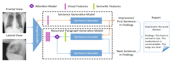
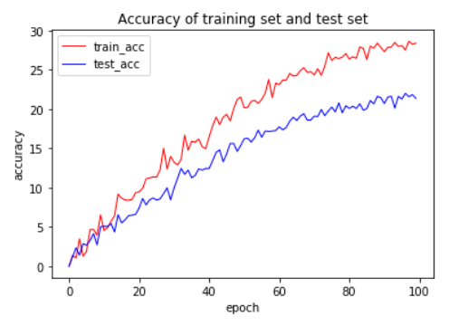
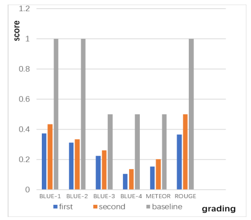
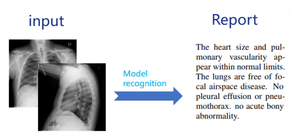
With the development of medical informatization and against the background of the spread of global epidemic, the demand for automated chest X-ray detection by medical personnel and patients continues to increase. Although the rapid development of deep learning technology has made it possible to automatically generate a single conclusive sentence, the results produced by existing methods are not reliable enough due to the complexity of medical images. To solve this problem, this paper proposes an improved RCLN (Recurrent Learning Network) model as a solution. The model can generate high-level conclusive impressions and detailed descriptive findings sentence-by-sentence and realize the imitation of the doctoros standard tone by combining a convolutional neural network (CNN) with a long short-term memory (LSTM) network through a recurrent structure, and adding a multi-head attention mechanism. The proposed algorithm has been experimentally verified on publicly available chest X-ray images from the Open-i image set. The results show that it can effectively solve the problem of automatic generation of colloquial medical reports.
Citation: Hui Li, Xintang Liu, Dongbao Jia, Yanyan Chen, Pengfei Hou, Haining Li. Research on chest radiography recognition model based on deep learning[J]. Mathematical Biosciences and Engineering, 2022, 19(11): 11768-11781. doi: 10.3934/mbe.2022548
With the development of medical informatization and against the background of the spread of global epidemic, the demand for automated chest X-ray detection by medical personnel and patients continues to increase. Although the rapid development of deep learning technology has made it possible to automatically generate a single conclusive sentence, the results produced by existing methods are not reliable enough due to the complexity of medical images. To solve this problem, this paper proposes an improved RCLN (Recurrent Learning Network) model as a solution. The model can generate high-level conclusive impressions and detailed descriptive findings sentence-by-sentence and realize the imitation of the doctoros standard tone by combining a convolutional neural network (CNN) with a long short-term memory (LSTM) network through a recurrent structure, and adding a multi-head attention mechanism. The proposed algorithm has been experimentally verified on publicly available chest X-ray images from the Open-i image set. The results show that it can effectively solve the problem of automatic generation of colloquial medical reports.

| [1] | Q. Z. You, H. L. Jin, Z. W. Wang, C. Fang, J. Luo, Image captioning with semantic attention, in Proceedings of the IEEE Conference on Computer Vision and Pattern Recognition, (2016), 4651–4659. https://doi.org/10.1109/CVPR.2016.336 |
| [2] | J. Krause, J. Johnson, R. Krishna, F. F. Li, A hierarchical approach for generating descriptive image paragraphs, in Proceedings of the IEEE Conference on Computer Vision and Pattern Recognition (CVPR), (2017), 3337–3346. https://doi.org/10.1109/CVPR.2017.356 |
| [3] |
R. K. Meleppat, L. K. Seah, M. V. Matham, Spectral phase-based automatic calibration scheme for swept source-based optical coherence tomography systems, Phys. Med. Biol., 61 (2016), 7652–7663. https://doi.org/10.1117/12.2190530 doi: 10.1117/12.2190530

|
| [4] |
R. K. Meleppat, In vivo multimodal retinal imaging of disease-related pigmentary changes in retinal pigment epithelium, Sci. Rep., 11 (2021), 1–14. https://doi.org/10.1088/0031-9155/61/21/7652 doi: 10.1088/0031-9155/61/21/7652
|
| [5] |
R. K. Meleppat, Plasmon resonant silica-coated silver nanoplates as contrast agents for optical coherence tomography, J. Biomed. Nanotechnol., 12 (2016), 1929–1937. https://doi.org/10.1166/jbn.2016.2297 doi: 10.1166/jbn.2016.2297
|
| [6] |
S. Hochreiter, J. Schmidhuber, Long short-term memory, Neural Comput., 9 (1997), 1735–1780. http://doi:10.1162/neco.1997.9.8.1735 doi: 10.1162/neco.1997.9.8.1735
|
| [7] | H. Fang, S. Gupta, F. Iandola, R. K. Srivastava, L. Deng, P. Dollár, et al., From captions to visual concepts and back, in Proceedings of the IEEE conference on computer vision and pattern recognition, (2015), 1473–1482. https://doi.org/10.1109/CVPR.2015.7298754 |
| [8] | K. Andrej, F. F. Li, Deep visual semantic alignments for generating image descriptions, in Proceedings of the IEEE Conference on Computer Vision and Pattern Recognition, (2015), 3128–3137. https://doi.org/10.1109/TPAMI.2016.2598339 |
| [9] | H. Bierens, The Nadaraya-Watson kernel regression function estimator, in Topics in Advanced Econometrics: Estimation, Testing, and Specification of Cross-Section and Time Series Models, (1994), 212–247. https://doi.org/10.1017/CBO9780511599279.011 |
| [10] |
X. Wang, Z. Duan, L. Liu, M. Li, Y. An, Y. Zhou, Multi-Timescale load forecast of large power customers based on online data recovery and time series neural networks, J. Circuits Syst. Comput., 31 (2022), 2250088. https://doi.org/10.1142/S0218126622500888 doi: 10.1142/S0218126622500888
|
| [11] |
S. Wang, X. Ye, Y. Gu, J. Wang, Y. Meng, J. Tian, et al., Multi-label semantic feature fusion for remote sensing image captioning, ISPRS J. Photogramm. Remote Sens., 2022 (2022), 1–18. https://doi.org/10.1016/j.isprsjprs.2021.11.020 doi: 10.1016/j.isprsjprs.2021.11.020
|
| [12] |
F. Christophe, Learning algorithm recommendation framework for IS and CPS security: Analysis of the RNN, LSTM, and GRU contributions, Int. J. Syst. Software Secur. Prot., 13 (2022), 1–8. https://doi.org/10.4018/IJSSSP.293236 doi: 10.4018/IJSSSP.293236
|
| [13] |
G. Tong, Y. Li, D. Chen, Q. Sun, W. Cao, G. Xiang, CSPC-Dataset: New LiDAR point cloud dataset and benchmark for large-scale semantic segmentation, IEEE Access, 8 (2020), 87695–87718. https://doi.org/10.1109/ACCESS.2020.2992612 doi: 10.1109/ACCESS.2020.2992612
|
| [14] | J. Lei, L. Wang, Y. Shen, D. Yu, T. L. Berg, M. Bansal, MART: Memory-augmented recurrent transformer for coherent video paragraph captioning, preprint, arXiv: 2005.05402. |
| [15] | Z. F. Li, Y. Q. Yang, L. P. Wu, Study of text sentiment analysis method based on GA-CNN-LSTM model, J. Jiangsu Ocean Univ. (Nat. Sci. Ed.), 30 (2021), 79–86. |
| [16] |
H. Li, X. P. Ma, J. Shi, C. Li, Z. Zhong, H. Cai, A recommendation model by means of trust transition in complex network environment, Acta Autom. Sin., 44 (2018), 363–376. https://doi.org/10.16383/j.aas.2018.c160395 doi: 10.16383/j.aas.2018.c160395
|
| [17] |
Y. Ma, P. Feng, P. He, Y. Ren, X. Guo, X. Yu, et al., Segmenting lung lesions of COVID-19 from CT images via pyramid pooling improved Unet, Biomed. Phys. Eng. Express, 7 (2021), 45008. https://doi.org/10.1088/2057-1976/ac008a doi: 10.1088/2057-1976/ac008a
|
| [18] |
H. Y. Chung, Automatische evaluation der Humanübersetzung: BLEU vs. METEOR, Lebende Sprachen, 65 (2020), 25–36. https://doi.org/10.1515/les-2020-0009 doi: 10.1515/les-2020-0009
|
| [19] |
C. Zhao, Y. Xu, Z. He, J. Tang, Y. Zhang, J. Han, et al., A new approach for lung segmentation and automatic detection of COVID-19 using radiomic features from chest CT images, Pattern Recognit., 119 (2021), 108071–108079. https://doi.org/10.1016/j.patcog.2021.108071 doi: 10.1016/j.patcog.2021.108071
|
| [20] |
S. A. Thorat, K. P. Jadhav, Improving conversation modelling using attention based variational hierarchical RNN, Int. J. Comput., 20 (2021), 39–45. https://doi.org/10.47839/ijc.20.1.2090 doi: 10.47839/ijc.20.1.2090
|
| [21] |
H. M. Sabbir, Att-BiL-SL: Attention-based Bi-LSTM and sequential LSTM for describing video in the textual formation, Appl. Sci., 12 (2021), 1–8. https://doi.org/10.3390/app12010317 doi: 10.3390/app12010317
|
| [22] |
N. Mu, H. Y. Wang, Y. Zhang, J. Jiang, J. Tang, Progressive global perception and local polishing network for lung infection segmentation of COVID-19 CT images, Pattern Recognit., 120 (2021), 108168. https://doi.org/10.1016/j.patcog.2021.108168 doi: 10.1016/j.patcog.2021.108168
|
| [23] |
X. Liu, Q. Yuan, Y. Gao, K. He, S. Wang, X. Tang, et al., Weakly supervised segmentation of COVID-19 Infection with scribble annotation on CT images, Pattern Recognit., 122 (2022), 108341–108349. https://doi.org/10.1016/j.patcog.2021.108341 doi: 10.1016/j.patcog.2021.108341
|
| [24] |
J. He, Q. Zhu, K. Zhang, P. Yu, J. Tang, An evolvable adversarial network with gradient penalty for COVID-19 infection segmentation, Appl. Soft Comput., 113 (2021), 107947–107956. https://doi.org/10.1016/j.asoc.2021.107947 doi: 10.1016/j.asoc.2021.107947
|
| [25] |
D. Deutsch, T. B Weiss, D. Roth, Towards question-answering as an automatic metric for evaluating the content quality of a summary, Trans. Assoc. Comput. Linguist., 9 (2021), 774–789. https://doi.org/10.1162/TACL_A_00397 doi: 10.1162/TACL_A_00397
|
| [26] |
F. P Martin, H. Weishaar, F. Cristea, J. Hanefeld, L. Schaade, C. E. Bcheraoui, Impact of type and timeliness of public health policies on COVID-19 epidemic growth: Organization for economic co-operation and development (OECD) member states, January–July 2020, SSRN Electron. J., 2020 (2020), 1–8. https://doi.org/10.2139/ssrn.3698853 doi: 10.2139/ssrn.3698853
|
| [27] |
Y. Lecun, L. Bottou, Gradient-based learning applied to document recognition, Proc. IEEE, 86 (1998), 2278–2324. https://doi.org/10.1109/5.726791 doi: 10.1109/5.726791
|
| [28] |
R. J. Williams, D. Zipser, A learning algorithm for continually running fully recurrent neural networks, Neural Comput., 1 (1989), 270–280. https://doi.org/10.1162/neco.1989.1.2.270 doi: 10.1162/neco.1989.1.2.270
|
| [29] |
D. Buchan, D. T. Jones, Learning a functional grammar of protein domains using natural language word embedding techniques, Proteins Struct. Funct. Bioinf., 88 (2020), 2555. https://doi.org/10.1002/prot.25842 doi: 10.1002/prot.25842
|
| [30] |
D. Jia, Y. Fujishita, C. Li, Y. Todo, H. Dai, Validation of large-scale classification problem in dendritic neuron model using particle antagonism mechanism, Electronics, 9 (2020), 792. https://doi.org/10.3390/electronics9050792 doi: 10.3390/electronics9050792
|
| [31] | X. G. Lv, X. M. Sun, G. L. Zhu, L. Jiang, S. T. Lu, Research on image smoothing and texture extraction based on variational method, J. Jiangsu Ocean Univ. (Nat. Sci. Ed.), 30 (2021), 77–84. |
Figures(7) / Tables(1)

Hui Li, Xintang Liu, Dongbao Jia, Yanyan Chen, Pengfei Hou, Haining Li. Research on chest radiography recognition model based on deep learning[J]. Mathematical Biosciences and Engineering, 2022, 19(11): 11768-11781. doi: 10.3934/mbe.2022548


 DownLoad: