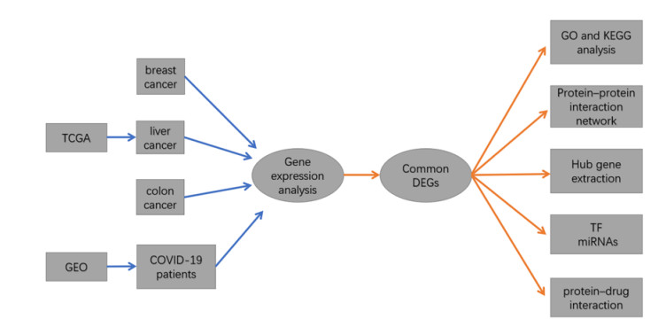
Figure 1.
Flowchart for research into bioinformatics data from The Gene Expression Omnibus (GEO) and The Cancer Genome Atlas (TCGA) database.


Severe acute respiratory syndrome coronavirus type 2 (SARS-CoV-2), also known as COVID-19, is currently prevalent worldwide and poses a significant threat to human health. Individuals with cancer may have an elevated risk for SARS-CoV-2 infections and adverse outcomes. Therefore, it is necessary to explore the internal relationship between these two diseases. In this study, transcriptome analyses were performed to detect mutual pathways and molecular biomarkers in three types of common cancers of the breast, liver, colon, and COVID-19. Such analyses could offer a valuable understanding of the association between COVID-19 and cancer patients. In an analysis of RNA sequencing datasets for three types of cancers and COVID-19, we identified a sum of 38 common differentially expressed genes (DEGs). A variety of combinational statistical approaches and bioinformatics techniques were utilized to generate the protein-protein interaction (PPI) network. Subsequently, hub genes and critical modules were found using this network. In addition, a functional analysis was conducted using ontologies keywords, and pathway analysis was also performed. Some common associations between cancer and the risk and prognosis of COVID-19 were discovered. The datasets also revealed transcriptional factors-gene interplay, protein-drug interaction, and a DEGs-miRNAs coregulatory network with common DEGs. The potential medications discovered in this investigation could be useful in treating cancer and COVID-19.
Citation: Qinyan shen, Jiang wang, Liangying zhao. To investigate the internal association between SARS-CoV-2 infections and cancer through bioinformatics[J]. Mathematical Biosciences and Engineering, 2022, 19(11): 11172-11194. doi: 10.3934/mbe.2022521
| [1] | Miao Zhu, Tao Yan, Shijie Zhu, Fan Weng, Kai Zhu, Chunsheng Wang, Changfa Guo . Identification and verification of FN1, P4HA1 and CREBBP as potential biomarkers in human atrial fibrillation. Mathematical Biosciences and Engineering, 2023, 20(4): 6947-6965. doi: 10.3934/mbe.2023300 |
| [2] | Ahmed Hammad, Mohamed Elshaer, Xiuwen Tang . Identification of potential biomarkers with colorectal cancer based on bioinformatics analysis and machine learning. Mathematical Biosciences and Engineering, 2021, 18(6): 8997-9015. doi: 10.3934/mbe.2021443 |
| [3] | Fang Niu, Zongwei Liu, Peidong Liu, Hongrui Pan, Jiaxue Bi, Peng Li, Guangze Luo, Yonghui Chen, Xiaoxing Zhang, Xiangchen Dai . Identification of novel genetic biomarkers and treatment targets for arteriosclerosis-related abdominal aortic aneurysm using bioinformatic tools. Mathematical Biosciences and Engineering, 2021, 18(6): 9761-9774. doi: 10.3934/mbe.2021478 |
| [4] | A. D. Al Agha, A. M. Elaiw . Global dynamics of SARS-CoV-2/malaria model with antibody immune response. Mathematical Biosciences and Engineering, 2022, 19(8): 8380-8410. doi: 10.3934/mbe.2022390 |
| [5] | Tingting Chen, Wei Hua, Bing Xu, Hui Chen, Minhao Xie, Xinchen Sun, Xiaolin Ge . Robust rank aggregation and cibersort algorithm applied to the identification of key genes in head and neck squamous cell cancer. Mathematical Biosciences and Engineering, 2021, 18(4): 4491-4507. doi: 10.3934/mbe.2021228 |
| [6] | Wenhan Guo, Yixin Xie, Alan E Lopez-Hernandez, Shengjie Sun, Lin Li . Electrostatic features for nucleocapsid proteins of SARS-CoV and SARS-CoV-2. Mathematical Biosciences and Engineering, 2021, 18(3): 2372-2383. doi: 10.3934/mbe.2021120 |
| [7] | A. M. Elaiw, Raghad S. Alsulami, A. D. Hobiny . Global dynamics of IAV/SARS-CoV-2 coinfection model with eclipse phase and antibody immunity. Mathematical Biosciences and Engineering, 2023, 20(2): 3873-3917. doi: 10.3934/mbe.2023182 |
| [8] | Jie Wang, Md. Nazim Uddin, Rehana Akter, Yun Wu . Contribution of endothelial cell-derived transcriptomes to the colon cancer based on bioinformatics analysis. Mathematical Biosciences and Engineering, 2021, 18(6): 7280-7300. doi: 10.3934/mbe.2021360 |
| [9] | Dong-feng Li, Aisikeer Tulahong, Md. Nazim Uddin, Huan Zhao, Hua Zhang . Meta-analysis identifying epithelial-derived transcriptomes predicts poor clinical outcome and immune infiltrations in ovarian cancer. Mathematical Biosciences and Engineering, 2021, 18(5): 6527-6551. doi: 10.3934/mbe.2021324 |
| [10] | Peng Gu, Dongrong Yang, Jin Zhu, Minhao Zhang, Xiaoliang He . Bioinformatics analysis identified hub genes in prostate cancer tumorigenesis and metastasis. Mathematical Biosciences and Engineering, 2021, 18(4): 3180-3196. doi: 10.3934/mbe.2021158 |
Severe acute respiratory syndrome coronavirus type 2 (SARS-CoV-2), also known as COVID-19, is currently prevalent worldwide and poses a significant threat to human health. Individuals with cancer may have an elevated risk for SARS-CoV-2 infections and adverse outcomes. Therefore, it is necessary to explore the internal relationship between these two diseases. In this study, transcriptome analyses were performed to detect mutual pathways and molecular biomarkers in three types of common cancers of the breast, liver, colon, and COVID-19. Such analyses could offer a valuable understanding of the association between COVID-19 and cancer patients. In an analysis of RNA sequencing datasets for three types of cancers and COVID-19, we identified a sum of 38 common differentially expressed genes (DEGs). A variety of combinational statistical approaches and bioinformatics techniques were utilized to generate the protein-protein interaction (PPI) network. Subsequently, hub genes and critical modules were found using this network. In addition, a functional analysis was conducted using ontologies keywords, and pathway analysis was also performed. Some common associations between cancer and the risk and prognosis of COVID-19 were discovered. The datasets also revealed transcriptional factors-gene interplay, protein-drug interaction, and a DEGs-miRNAs coregulatory network with common DEGs. The potential medications discovered in this investigation could be useful in treating cancer and COVID-19.
On March 11, 2020, the World Health Organization (WHO) proclaimed the novel coronavirus outbreak, popularly known as SARS-CoV-2, a global pandemic [1]. As indicated by WHO (https://covid19.who.int/), the SARS-CoV-2 mortality rate is around 1.36%, with around 440,807,756 confirmed cases, including 5,978,096 deaths by March 2022 [2]. Studies have indicated that cancer patients have a greater vulnerability to SARS-CoV-2 infection caused by chemotherapy or immunotherapy [3]. In a large population sample study of more than 20,000 cancer patients, it was found that there was a significant increase in the SARS-CoV-2 infection among cancer patients [3]. According to recent studies, Individuals with cancer exhibited a greater likelihood of developing serious complications (such as intensive care unit hospitalization, invasive ventilation, or death) as opposed to those who did not have cancer (39 vs. 8%, p = 0·0003) [4]. With the advancement of medical science and tumor treatment methods in recent decades, the survival rate of cancer patients has continuously increased, and cancer is now considered a chronic disease rather than a terminal disease [5]. However, immunocompromised patients are at high risk as SARS-CoV-2 continues to mutate. Therefore, to better overcome these two diseases in the future, it is urgent to explore and clarify the internal molecular mechanism between them.
In this study, we selected breast cancer, liver cancer, and colon cancer, to explore the molecular mechanism between these three cancers and COVID-19. We chose breast cancer, liver cancer and colon cancer for analysis mainly for the following three reasons: 1) According to February 2022, the National Cancer Center of China announced the incidence of cancer in China in 2016 [6]. The current top five cancers are lung cancer, colon cancer, gastric cancer, liver cancer, and breast cancer. Therefore, there are a certain representative. 2) With the progress of surgical operations and the continuous development of comprehensive diagnosis and treatment of tumors, the overall prognosis of these three cancers (breast cancer liver cancer and colon cancer) is good at present. In our clinical work, we have found that many patients have been cured or have stable survival with tumor after undergoing surgery, radiotherapy and chemotherapy, immunotherapy and other treatments. However, gastric cancer patients have poor prognosis and low long-term survival rate. In our opinion, cancer will no longer be an incurable disease in the future, but will evolve into chronic diseases such as hypertension and diabetes. Therefore, we may have a greater chance of encountering these three types of cancer patients with COVID-19 in the long-term clinical practice. 3) The reason why we did not include lung cancer is that SARS-CoV-2 virus mainly affects lung, and the two diseases are in the same target organ. In our opinion, they need to be analyzed separately. We first identified the differentially expressed genes (DEGs) for the three distinct malignancies and the SARS-CoV-2 virus to discover the DEGs shared by all four disorders. This research is focused on the common DEGs, which serve as the core experimental genes. Additional investigations and analyses were carried out on the basis of these common DEGs and included a pathway analysis and an enrichment analysis to truly comprehend the biological mechanisms behind genome-based expression investigations. The extraction of hub genes from common DEGs was a critical step in the prediction of viable medicines. In addition, a network of protein-protein interactions (PPIs) was constructed using common DEGs to collect hub genes for further study. In this research, transcription modulators were identified predicated on the common DEGs. Last but not least, possible medications were proposed. The detailed procedure of our study is shown in Figure 1.
The transcriptome data of three common cancers of the breast, colon, and liver were acquired from The Cancer Genome Atlas (TCGA) database (https://portal.gdc.cancer.gov/). These include 1222 breast specimens (1109 cancer specimens, 113 normal tissue specimens), 546 colon specimens (502 cancer specimens, 44 normal tissue specimens), and 424 liver specimens (374 cancer specimens, 50 normal tissue specimens). The SARS-CoV-2 infection data were obtained from The Gene Expression Omnibus (GEO) database (ID: GSE147507) of the National Center for Biotechnology Information (NCBI) (https://www.ncbi.nlm.nih.gov/geo/) [7].
A statistically significant difference between distinct test settings at the transcriptional level was used as the criterion for determining genes that are differently expressed. Long-expression levels for DEGs were discovered utilizing the "limma" program with the Benjamini-Hochberg correction to adjust the false discovery rate. "DESEq2" of the R programming language (v 4.0.2) was also used to identify DEGs under a variety of testing settings. A p-value < 0.05 and |logFC| ≥1.0 was considered to be statistically significant. The common DEGs from four datasets were obtained by utilizing an online Venn analysis program known as Jvenn [8].
A gene set enrichment analysis is a substantial analytical endeavor that aims to categorize basic biological knowledge, including cellular mechanisms of chromosomal sites related to several interconnected disorders [9]. Enrichr (https://maayanlab.cloud/Enrichr/) was utilized to conduct gene ontology, functional enrichment (cellular components (CC), biological processes (BP), and molecular functions (MF)), and pathway enrichment investigations. Enrichr is a web-based program for enriching gene sets [10] that is employed to study the biological processes and signaling paths underlying common DEGs. A total of four repositories were investigated for this research: the Kyoto Encyclopedia of Genes and Genomes (KEGG), BioCarta, Reactome and WikiPathways. These highlighted the genesis of the route categorization, which was used to identify the pathways shared by breast cancer, colon cancer, liver cancer, and COVID-19. Notably, the KEGG pathway is well recognized for its ability to comprehend metabolic processes while also demonstrating the significant value of genomic research. The standard criterion for measuring the top-listed pathways was a p-value < 0.05.
We then investigated the interactive relationships between proteins utilizing STRING (Search Tool for the Retrieval of Interacting Genes/Proteins), a web-based program that can be retrieved at https://string-db.org/. The use of STRING to study the PPI network of DEGs may aid in examining the associations across various genes. The STRING repository was utilized to create the PPI network of proteins generated from common DEGs in order to depict physical and functional relationships across three distinct cancer types and SARS-CoV-2. Hereafter, Cytoscape (v.3.7.1) was used to visualize and conduct subsequent investigations on the PPI network once it was loaded into the program. Cytoscape, a publicly accessible network visualization tool, is a versatile system in which multiple datasets are integrated to optimize for diverse interactions including PPIs, genetic connections, protein-DNA interplay, and so on. The PPI network is composed of edges, nodes, and interconnections between them. In this context, the nodes that are the most entangled are referred to be the hub genes. Cytohubba (https://apps.cytoscape.org/apps/cytohubba), a revolutionary Cytoscape plugin, is a tool for ranking and isolating central, potential, or targeted components of a biological network depending on a variety of network characteristics. Cytohubba is a collection of 11 techniques for evaluating networks from a variety of perspectives. Maximal Clique Centrality (MCC) is considered the most effective method [11]. The PPI network's top ten hub genes were discovered using the MCC approach, which was applied to the network. According to Cytohubba's near proximity ranking characteristics, the shortest accessible pathways linking hub genes were also identified.
Transcriptional factors (TFs) are proteins capable of binding to a specific gene and regulating the rate at which genetic information is transcribed. As a result, it is necessary to provide molecular understandings. The NetworkAnalyst (http://www.networkanalyst.ca) platform was utilized to discover topologically credible TFs from the JASPAR database (http://jaspar.genereg.net) that have a tendency to bind to common DEGs. NetworkAnalyst is a robust web-based resource for meta-analysis of gene expression profiles and the discovery of biological processes, functions, and interpretations of those findings [12]. JASPAR is a freely accessible repository of TFs from six taxonomic categories that may be used to identify TFs in numerous species [13]. MiRNAs that target gene interactions were also incorporated in the research to identify miRNAs that have the potential to bind to gene transcripts and so negatively impact protein production. MiRTarBase and TarBase are two of the most important repositories for evaluating the experimental validity of miRNA-target gene interplay [14]. MiRNAs from miRTarBase and TarBase that interplay with common DEGs were retrieved from the interactions between miRNAs and genes utilizing NetworkAnalyst, with a particular emphasis on topological analysis. In Cytoscape, interaction networks between transcription factors and genes and between microRNAs and genes were shown. This program assists researchers in filtering top miRNAs exhibiting elevated levels of expression and identifying biological roles and characteristics that may be used to develop a reliable biological hypothesis.
The most significant impact of this research is predicting protein-drug interaction (PDI) or identifying drug molecules. Utilizing Drug Signatures Database (DSigDB) via Enrichr, a drug molecule was discovered on the basis of the DEGs of SARS-CoV-2 and three distinct subtypes of cancer. DSigDB is a worldwide library for identifying targeted pharmacological compounds that are associated with DEGs [15]. Enrichr's "Diseases/Drugs" feature provides easy access to this database, which comprises 22,527 gene sets.
The datasets analyzed during the present study are available from The Cancer Genome Atlas (TCGA) database (https://portal.gdc.cancer.gov/) and The Gene Expression Omnibus (GEO) database of the National Center for Biotechnology Information (NCBI) (https://www.ncbi.nlm.nih.gov/geo/).
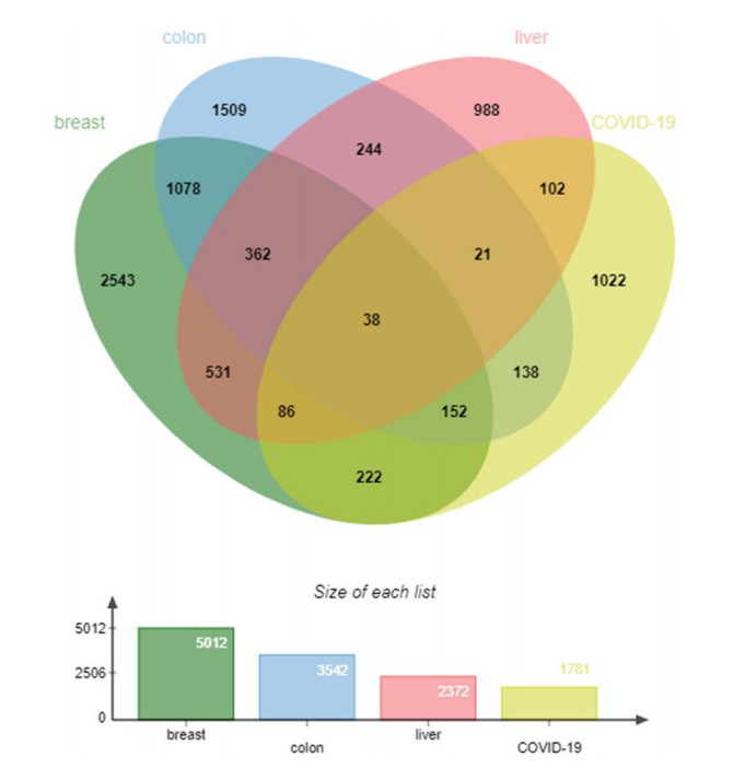
In this research, 1,781 genes were found to have a differential expression for COVID-19, where 391 were up-modulated and 1390 were down-modulated. From the assessment of TCGA data, 5012 DEGs (1997 up-modulated and 3015 down-modulated) were discovered in the breast cancer dataset, 3542 DEGs (1374 up-modulated and 2168 down-modulated) in the colon cancer data, and 2372 DEGs (979 up-modulated and 1393 down-modulated) in the liver cancer data. All of the significant DEGs were identified based on a p-value < 0.05 and |logFC| ≥ 1. Table 1 provides a summary of the information included within the datasets. Following the execution of the cross-comparison evaluation on Jvenn, 38 common DEGs were discovered from breast cancer, colon cancer, liver cancer, and COVID-19 datasets. Further analysis of these common genes was performed. All showed that all three cancers are linked to COVID-19 since they share one or more common genes. Figure 2 depicts the cumulative comparison study of the four datasets, as well as the extraction of the common DEGs.
| Disease name | Data sources | Total DEGs count | Up-modulated DEGs count | Down-modulated DEGs count |
| COVID-19 | GEO | 1781 | 391 | 1390 |
| Breast cancer | TCGA | 5012 | 1997 | 3015 |
| Colon cancer | TCGA | 3542 | 1374 | 2168 |
| Liver cancer | TCGA | 2372 | 979 | 1393 |
 DownLoad:
CSV
DownLoad:
CSV
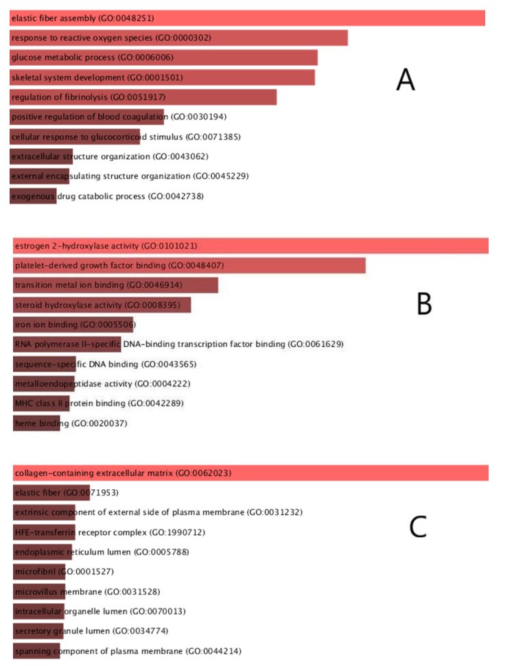
Enrichr was used to conduct GO and KEGG enrichment analyses of the common DEGs in order to determine their biological value and the enriched pathways behind them. The GO analysis was determined within three categories (BP, CC and MF). As a source for annotating data, the GO database was used. Table 2 summarizes the top ten terms in the BP, MF, and CC categories. The bar graph in Figure 3 demonstrates the complete ontological analysis in a linear manner for each of the different categories.
| Category | GO ID | Term | P-value | Genes |
| GO biological process | GO: 0048251 | elastic fiber assembly | 9.77 × 10⁻⁵ | MFAP4; TNXB |
| GO: 0000302 | response to reactive oxygen species | 0.000191 | APOD; FOS; MMP9 | |
| GO: 0006006 | glucose metabolic process | 0.000221 | APOD; PCK1; PPARGC1A | |
| GO: 0001501 | skeletal system development | 0.000225 | COL2A1;COL1A2;IHH; PITX1 | |
| GO: 0051917 | regulation of fibrinolysis | 0.000271 | F12; HRG | |
| GO: 0030194 | positive regulation of blood coagulation | 0.00047 | F12; HRG | |
| GO: 0071385 | cellular response to glucocorticoid stimulus | 0.000528 | ZFP36; PCK1 | |
| GO: 0043062 | extracellular structure organization | 0.000732 | MMP11; COL2A1; COL1A2; MMP9 | |
| GO: 0045229 | external encapsulating structure organization | 0.000745 | MMP11; COL2A1; COL1A2; MMP9 | |
| GO: 0042738 | exogenous drug catabolic process | 0.000793 | CYP2B6; CYP3A4 | |
| GO cellular component | GO: 0062023 | collagen-containing extracellular matrix | 2.94 × 10⁻⁸ | MFAP4; ECM1; TNXB; COL2A1; COL1A2; F12; HRG; MMP9; ANGPTL1 |
| GO: 0071953 | elastic fiber | 0.009465 | MFAP4 | |
| GO: 0031232 | extrinsic component of external side of plasma membrane | 0.015102 | TF | |
| GO: 1990712 | HFE-transferrin receptor complex | 0.015102 | TF | |
| GO: 0005788 | endoplasmic reticulum lumen | 0.016724 | TF; COL2A1; COL1A2 | |
| GO: 0001527 | microfibril | 0.020708 | MFAP4 | |
| GO: 0031528 | microvillus membrane | 0.020708 | CDHR2 | |
| GO: 0070013 | intracellular organelle lumen | 0.021331 | MMP11; TF; COL2A1; COL1A2; MMP9 | |
| GO: 0034774 | secretory granule lumen | 0.021924 | ECM1; TF; HRG | |
| GO: 0044214 | spanning component of plasma membrane | 0.024427 | CDHR2 | |
| GO molecular function | GO: 0101021 | estrogen 2-hydroxylase activity | 3.5 × 10⁻⁵ | CYP2B6; CYP3A4 |
| GO: 0048407 | platelet-derived growth factor binding | 0.000191 | COL1A2; COL2A1 | |
| GO: 0046914 | transition metal ion binding | 0.001461 | RGN; CYP3A4; PCK1; HRG; MMP9 | |
| GO: 0008395 | steroid hydroxylase activity | 0.002126 | CYP2B6; CYP3A4 | |
| GO: 0005506 | iron ion binding | 0.004727 | TF; CYP3A4 | |
| GO: 0061629 | RNA polymerase Ⅱ-specific DNA-binding transcription factor binding | 0.005576 | FOS; PITX1; PPARGC1A | |
| GO: 0043565 | sequence-specific DNA binding | 0.010403 | CSRNP1; TBX15; FOS; PITX1; PPARGC1A | |
| GO: 0004222 | metalloendopeptidase activity | 0.010609 | MMP11; MMP9 | |
| GO: 0042289 | MHCclass Ⅱ protein binding | 0.011347 | COL2A1 | |
| GO: 0020037 | heme binding | 0.012942 | CYP2B6; HRG | |
| *Note: Top 10 terms of each category are listed. | ||||
DownLoad:
CSV
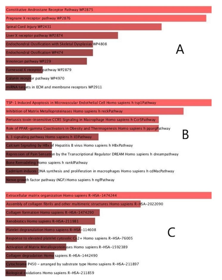
It was discovered via a pathway analysis that the organism has a reaction with its inherent alterations. In order to identify the most significantly altered pathways of the common DEGs in breast cancer, colon cancer, liver cancer, and COVID-19, four universal databases were used, including Reactome, WikiPathways, KEGG and Biocarta. Table 3 contains a summary of the most important pathways discovered via the analysis of the specified datasets. Furthermore, the pathway enrichment study is depicted in the bar charts in Figure 4.
| category | Term | P-value | Genes |
| WikiPathways | Constitutive Androstane Receptor Pathway WP2875 | 3.02 × 10⁻⁵ | CYP2B6; CYP3A4; PPARGC1A |
| Pregnane X receptor pathway WP2876 | 3.32 × 10⁻⁵ | CYP2B6; CYP3A4; PPARGC1A | |
| Spinal Cord Injury WP2431 | 7.28 × 10⁻⁵ | ZFP36; COL2A1; FOS; MMP9 | |
| Liver X receptor pathway WP2874 | 0.000157 | CYP2B6; CYP3A4 | |
| Endochondral Ossification with Skeletal Dysplasias WP4808 | 0.000243 | COL2A1; IHH; MMP9 | |
| Endochondral Ossification WP474 | 0.000243 | COL2A1; IHH; MMP9 | |
| Irinotecan pathway WP229 | 0.000271 | BCHE; CYP3A4 | |
| Farnesoid X receptor pathway WP2879 | 0.000589 | CYP3A4; PPARGC1A | |
| Galanin receptor pathway WP4970 | 0.000722 | FOS; PPARGC1A | |
| miRNA targets in ECM and membrane receptors WP2911 | 0.000793 | TNXB; COL1A2 | |
| BioCarta | TSP-1 Induced Apoptosis in Microvascular Endothelial Cell Homo sapiens h tsp1Pathway | 0.013226 | FOS |
| Inhibition of Matrix Metalloproteinases Homo sapiens h reckPathway | 0.015102 | MMP9 | |
| Pertussis toxin-insensitive CCR5 Signaling in Macrophage Homo sapiens h Ccr5Pathway | 0.016974 | FOS | |
| Role of PPAR-gamma Coactivators in Obesity and Thermogenesis Homo sapiens h ppargPathway | 0.016974 | PPARGC1A | |
| IL 3 signaling pathway Homo sapiens h il3Pathway | 0.022569 | FOS | |
| Calcium Signaling by HBx of Hepatitis B virus Homo sapiens h HBxPathway | 0.028134 | FOS | |
| Repression of Pain Sensation by the Transcriptional Regulator DREAM Homo sapiens h dreampathway | 0.028134 | FOS | |
| Bone Remodeling Homo sapiens h ranklPathway | 0.029982 | FOS | |
| Cadmium induces DNA synthesis and proliferation in macrophages Homo sapiens h cdMacPathway | 0.029982 | FOS | |
| Nerve growth factor pathway (NGF) Homo sapiens h ngfPathway | 0.031826 | FOS | |
| Reactome | Extracellular matrix organization Homo sapiens R-HSA-1474244 | 1.44 × 10⁻⁵ | MMP11;MFAP4;TNXB; COL2A1; COL1A2; MMP9 |
| Assembly of collagen fibrils and other multimeric structures Homo sapiens R-HSA-2022090 | 0.000147 | COL2A1; COL1A2; MMP9 | |
| Collagen formation Homo sapiens R-HSA-1474290 | 0.000561 | COL2A1; COL1A2; MMP9 | |
| Xenobiotics Homo sapiens R-HSA-211981 | 0.000654 | CYP2B6; CYP3A4 | |
| Platelet degranulation Homo sapiens R-HSA-114608 | 0.001038 | ECM1; TF; HRG | |
| Response to elevated platelet cytosolic Ca2+ Homo sapiens R-HSA-76005 | 0.001187 | ECM1; TF; HRG | |
| Activation of Matrix Metalloproteinases Homo sapiens R-HSA-1592389 | 0.001682 | MMP11; MMP9 | |
| Collagen degradation Homo sapiens R-HSA-1442490 | 0.002492 | MMP11; MMP9 | |
| Cytochrome P450 - arranged by substrate type Homo sapiens R-HSA-211897 | 0.006187 | CYP2B6; CYP3A4 | |
| Biological oxidations Homo sapiens R-HSA-211859 | 0.006336 | CYP2B6; GLYATL1; CYP3A4 | |
| KEGG | ECM-receptor interaction | 0.000621 | TNXB; COL2A1; COL1A2 |
| Relaxin signaling pathway | 0.001875 | COL1A2; FOS; MMP9 | |
| PI3K-Akt signaling pathway | 0.004431 | TNXB; COL2A1;COL1A2; PCK1 | |
| Focal adhesion | 0.006513 | TNXB; COL2A1; COL1A2 | |
| Proteoglycans in cancer | 0.006876 | COL1A2; IHH; MMP9 | |
| Retinol metabolism | 0.0074 | CYP2B6; CYP3A4 | |
| Adipocytokine signaling pathway | 0.007611 | PCK1; PPARGC1A | |
| Lipid and atherosclerosis | 0.007835 | CYP2B6; FOS; MMP9 | |
| Metabolism of xenobiotics by cytochrome P450 | 0.00917 | CYP2B6; CYP3A4 | |
| Leishmaniasis | 0.009403 | FCGR3A; FOS | |
| *Note: Top 10 terms of each category are listed. | |||
DownLoad:
CSV
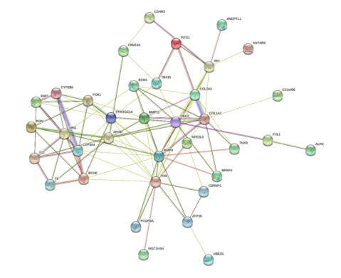
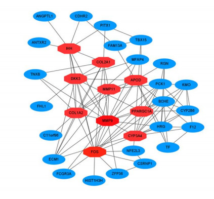
We examined the PPI network constructed from STRING and displayed it in Cytoscape in order to predict the interactions and adhesion routes of frequent DEGs. Figure 5 depicts the PPI network of common DEGs, which comprises 101 edges and 38 nodes. In a PPI network, the nodes with the most interconnections are interpreted to be hub genes. The topmost 10 DEGs were determined to be the most significant genes based on the PPI network analysis performed in Cytoscape utilizing the Cytohubba plugin. These hub genes comprised MMP9, FOS, COL1A2, COL2A1, DKK3, IHH, CYP3A4, PPARGC1A, MMP11 and APOD. The identified hub genes could be possible biomarkers for illnesses under investigation, and they may potentially lead to the development of novel treatment techniques. With this potential in mind, a submodule network was constructed using the Cytohubba plugin to gain a greater comprehension of the close interaction and vicinity of the hub genes. Figure 6 depicts the extended network of hub-gene connections resulting from the PPI network.
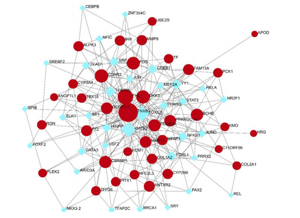
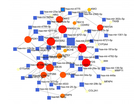
A network-based technique was used to decipher the modulatory TFs and miRNAs in order to discover significant modifications occurring at the transcription level and to gain knowledge of the regulatory molecules of hub genes or common DEGs. Figure 7 depicts the interplay of TFs and regulators with the common DEGs. Furthermore, Figure 8 depicts the interconnections of miRNA regulators with the common DEGs. Following the investigation of the TFs-gene and miRNAs-gene interactions networks, it was discovered that 72 TFs and 67 post-transcription (miRNAs) modulatory signatures interact with more than one common DEG. This simply suggests that there is a significant degree of crosstalk between them.
We then evaluated PDI in order to comprehend the structural characteristics that are indicated for the sensitivity of receptors. In the case of common DEGs as prospective therapeutic targets in cancer and COVID-19, Enrichr was used to identify ten candidate medicinal compounds that were on the basis of transcriptomic profiles from the DSigDB. The ten leading chemical substances were determined based on their p-values, and they were then extracted. These possible medications have been proposed as therapies for the common DEGs seen in cancer and COVID-19. Table 4 contains the drugs that are successful for these common DEGs that have been identified in the DSigDB database.
| Name | P-value | Molecular Formula |
| CHEMBL475540TTD 00006054 | 1.06 × 10⁻⁷ | C17H17NO6S |
| lycorine MCF7 UP | 2.54 × 10⁻⁷ | C16H17NO4 |
| astemizole MCF7 UP | 1.63 × 10⁻⁶ | C28H31FN4O |
| tamoxifen MCF7 UP | 1.73 × 10⁻⁶ | C26H29NO |
| azacitidine PC3 UP | 2.79 × 10⁻⁶ | C8H12N4O5 |
| azacyclonol MCF7 UP | 3.70 × 10⁻⁶ | C18H21NO |
| cycloheximide PC3 UP | 4.00 × 10⁻⁶ | C15H23NO4 |
| vanoxerine PC3 UP | 5.52 × 10⁻⁶ | C28H32F2N2O |
| mefloquine MCF7 UP | 7.68 × 10⁻⁶ | C17H16F6N2O |
| LY-294002 MCF7 UP | 7.98 × 10⁻⁶ | C19H17NO3 |
DownLoad:
CSV
The 2019 global pandemic of SARS-CoV-2 has become an emergency of major international concern. Growing evidence suggests that cancer patients have a greater vulnerability to this disease. In addition to having a greater susceptibility to this infection, cancer patients have a higher likelihood of advancing to a severe stage of SARS-CoV-2 than the general population[16,17]. Cancer is recognized as a pandemic, with over 18,000,000 individuals being diagnosed each year throughout the globe. The most comprehensive analysis from China includes data from 13,077 COVID-19 patients, among which 232 were found to develop cancer [18]. As a result, there will be more and more cancer patients developing SARS-CoV-2 infections in the years and decades to come. An increasing number of viruses and bacteria have been associated with human cancers [19]. To date, seven classes of viruses (Human papilloma virus (HPV), Hepatitis B virus (HBV), Hepatitis C virus (HCV), Kaposi's sarcoma associated herpesvirus (KSHV), Human T lymphotropic virus (HTLV), Merkel cell polyomavirus (MCpyV), Epstein Barr virus (EBV) have been identified to have oncogenic potential [20]. The oncoproteins of human tumor viruses regularly interact with the cellular epigenetic machinery. Such interactions alter the epigenome of the host cell and reprogram its gene expression pattern [21]. Helicobacter pylori is a bacterium known to be associated with gastroduodenal diseases such as chronic active gastritis, peptic ulcers, and gastric malignancies. Gene expression profiling in human gastric mucosa infected with Helicobacter pylori shows that host genes are dysregulated after Helicobacter pylori infection [22]. Some reports have studied the relationship between SARS-CoV-1 virus with the incidence of cancer. This virus which shares a lot of similarities with the SARS-CoV-2 virus has been reported to interfere with various signaling pathways associated with carcinogenic transformation of cells [23]. The genomic alterations of six SARS-CoV-2 receptor-related regulators (transmembrane serine protease 2 (TMPRSS2), angiotensinogen (AGT), angiotensin-converting enzyme 1 (ACE1), solute carrier family 6 member 19 (SLC6A19), angiotensin-converting enzyme 2 (ACE2), and angiotensin Ⅱ receptor type 2 (AGTR2)) and their clinical relevance across a broad spectrum of solid tumors were evaluated across 33 cancers [24]. Furthermore, four major similar signaling pathway, have been identified at the intersection of COVID-19 and cancer; namely, cytokine, type Ⅰ interferon (IFN-I), androgen receptor (AR), and immune checkpoint signaling [25]. In biomedical and system biology studies, expression profiling leveraging high throughput sequencing datasets is utilized to find biological marker candidates for various disorders [26]. In recent times, the capacity to analyze gene fusion, mutations/single nucleotide polymorphisms (SNPs), posttranscriptional alterations, and gene expression variations in diverse sets of therapies has been enhanced by RNA sequencing, a next-generation sequencing approach [27]. In this research, the transcriptome of three prevalent malignancies, as well as COVID-19, found that 38 common DEGs had comparable expression profiles. GO, and pathway enrichment studies on the basis of p-values were used to assess the biological significance of these common DEGs in order to comprehend the pathophysiology of four disorders. The GO analysis mainly included a biological process (BP, molecular activity), a cell component (CC, gene regulation function), and a molecular function (MF, molecular level activity). The common DEGs were mainly enriched in "elastic fiber assembly" (BP), "collagen-containing extracellular matrix" (CC), and "estrogen 2-hydroxylase activity" (MF). Furthermore, the analytical findings from KEGG enrichment illustrated the predominant involvement of common DEGs in the "ECM-receptor interaction", "relaxin signaling pathway", and "PI3K-Akt signaling pathway". Exploring these critical pathways could aid in the advancement of our knowledge of COVID-19 and the genesis of cancer. By using a network-based method, this research investigated the gene expression profiles in four RNA sequencing datasets of three common cancer types and COVID-19 patients. By analyzing patients the common phenotypic changes of cancer and COVID-19 patients, we hope to explore potential causative factors, and provide a theoretical basis for further study of these two diseases.
It is believed that a scarcity of specific medications is one of the primary causes of the continuing COVID-19 pandemic. We discovered the molecular targets that could be viable biological markers of cancer patients with SARS-CoV-2. A PPI network was constructed with the help of the DEG genes in order to truly comprehend the biological features of proteins and to explore therapeutic targets. In this study, 10 hub genes (MMP9, FOS, COL1A2, COL2A1, DKK3, IHH, CYP3A4, PPARGC1A, MMP11 and APOD) were examined, most of which were confirmed to be linked to the onset and progression of tumors in previous studies. Matrix metalloproteinases (MMPs) are endopeptidases with zinc (Zn2þ) as a cofactor that are found inside the cell and are bound by a biological membrane. MMP9 and MMP11 are two different forms of matrix metalloproteinases [28]. MMP-9 overexpression has been linked to a variety of malignancies, including breast, liver, and colon cancers [29,30,31,32]. Metallopeptidase activity affects respiratory disorders, including pulmonary fibrosis, acute lung injury, and acute respiratory distress syndrome (ARDS). MMP9 was previously found to be a significant biological marker of respiratory failure and SARS-CoV-2 infection in a prior investigation [33]. The FOS gene, which is found on chromosome 14q21–31 in humans, is responsible for encoding the nuclear oncoprotein c-Fos, the c-Fos protein binds to the c-Jun protein to generate a heterodimer (AP-1) that is capable of activating transcriptional activity. This is strongly linked to the proliferation and differentiation of cells, both of which contribute substantially to tumor transformation and reversal [34,35,36]. In the ECM-receptor pathway, the collagen type Ⅰ alpha 2 chain (COL1A2) performs a vital function and has been directly linked to the occurrence of diverse human malignancies [37]. DKK3 is a gene that inhibits tumor growth and its expression level has been shown to decrease in many kinds of cancers. DKK3 is a member of the DKK family (DKK1, DKK2, DKK3 and DKK4). It encodes for produced glycoproteins that are evolutionarily preserved and are made up of two unique cysteine-rich sites and act as an inhibitor of the oncogenic Wnt signaling pathway [38].The activation of the canonical Wnt/-catenin pathway in ARDS patients, particularly those with SARS-CoV-2, has been demonstrated to be linked to inflammatory and a cytokine storm, according to recent research [39,40]. However, whether the Wnt signaling pathway upregulation is the underlying molecular mechanism of cancer in patients with severe SARS-CoV-2 requires further investigation. Patients with lung adenocarcinoma and squamous cell carcinoma who had positive IHH expression had considerably shorter survival duration as opposed to those who had negative IHH expression, indicating that IHH is a prognostic factor for unsatisfactory prognosis [41]. CYP3A4, a member of the cytochrome P450 enzyme, is responsible for the metabolism of a wide range of anticancer drugs. Cancer patients with SARS-CoV-2 often require combination therapy, which can potentially lead to DDIs that result in an increased risk of side effects/toxicity or reduced effectiveness [42].Recently, Zulkar Naind et al. confirmed that PPARGC1A is a core protein implicated in SARS-CoV-2 infection as well as the risk factors associated with the disease [43].The study has shown that gene expression changes after infection with the SARS-CoV-2 [44]. Therefore, the hub genes that have been found may be used as prospective biological markers or, if the biological knowledge gained from SARS-CoV-2 is verified, as a new pharmacological target.
Moreover, TFs modulate the transcriptional ratio, whereas miRNA is a critical participant in RNA knockdown and gene expression control at the post-transcriptional level. As a result, both are necessary for understanding the progression mechanism of the illness. This research discovered links between the DEGs that were studied and their corresponding TFs and modulatory miRNAs. Several TFs were discovered, including STAT3, NFKB1, FOXC1, HINFP and JUN. There is evidence that these TFs are associated with viral-induced acute respiratory illnesses or the genesis and progression of malignancies [45,46,47,48]. Furthermore, several miRNAs play a role in breast cancer, (e.g. hsa-mir-335-5p, hsa-mir-139-5p, hsa-mir-25-3p, hsa-miR-32-3p) [49,50], liver cancer (e.g.hsa-mir-139-5p, hsa-mir-25-3p) [51,52], and colon cancer (e.g. hsa-mir-1301-3p, hsa-mir-29b-3p, hsa-mir-25-3p, hsa-mir-129-5p, hsa-miR-1277-5p) [53,54,55,56,57].There are several miRNAs involved in coronaviruses infection; for example, miRNAs were highly expressed in MERS-CoV-infected cells and may play important roles in disease development [58]. hsa-miR-139-5p can act as a risk factor for severe COVID-19 [59]. However, the role of miRNA in tumor patients with SARS-CoV-2 infection requires further research.
As per the latest report from WHO, no appropriate therapies or medicines for preventing and treating COVID-19 have been established and approved to date [2]. However, for years, several institutions, government agencies, research institutes, and pharmaceuticals have conducted clinical and preclinical studies to determine whether current medication moieties are effective in treating the disease on the basis of their prior experience with viral infections. In in vitro cell cultures, Wang et al. demonstrated that two medicines, remdesivir and chloroquine, were successful in managing SARS-CoV-2 infection [60]. Additionally, a clinical experiment revealed that the antibiotics azithromycin and hydroxychloroquine had a substantial impact on SARS-CoV-2 by interfering with its genome replication [61,62]. In this study, we identified several potential drugs to treat SARS-CoV-2 infection, such as lycorine and astemizole. Lycorine is a natural alkaloid that has been derived from the lycoris plant and has been shown to have a number of biological effects, such as antitumor, anti-viral, and anti-malaria activities [63,64]. Similarly, studies have shown that quartzine can reduce acute lung injury [65]. New research shows that astemizole may suppress the invasion of SARS-CoV-2 spike pseudoviruses by binding to the ACE2 receptor [66]. Therefore, these drugs are potential candidates for anti-coronavirus therapy.
In this study, the common differential genes of three different cancer types and COVID-19 patients were obtained through bioinformatics techniques. Additionally, the top 10 target genes were obtained through a PPI analysis of common differential genes. These target genes may be biomarkers for cancer or SARS-CoV-2 infection, which translates to potential drug targets. The association between these target genes and TFs and miRNAs was also studied to better understand their role in the occurrence and development of disease. Meanwhile, several targeted drugs with potential clinical value were identified for treating SARS-CoV-2 infection in patients with common types of cancer. Finally, our study uses public databases and bioinformatics analysis to find common genotype changes in cancer and COVID-19, but whether these genotype changes are potential causative factors of the two diseases, these potential gene targets and drugs can be further used in the clinic needs to be verified through experimental studies such as cells and animal models. This is the biggest deficiency in our research, and it is also the focus of our follow-up further research.
We would like to acknowledge the TCGA and GEO for providing data. This research received no external funding.
All authors declare no conflicts of interest in this paper.
| [1] |
D. Cucinotta, M. Vanelli, WHO Declares COVID-19 a Pandemic, Acta Biomed., 91 (2020), 157–160. https://doi.org/10.23750/abm.v91i1.9397 doi: 10.23750/abm.v91i1.9397

|
| [2] | World Health Organization, Coronavirus disease (COVID-19). Available from: https://covid19.who.int/. |
| [3] |
K. A. Lee, W. Ma, D. R. Sikavi, D. A. Drew, L. H. Nguyen, R. Bowyer, et al., Cancer and risk of COVID-19 through a general community survey, Oncologist, 26 (2021), e182–e185. https://doi.org/10.1634/theoncologist.2020-0572 doi: 10.1634/theoncologist.2020-0572
|
| [4] |
W. Liang, W. Guan, R. Chen, W. Wang, J. Li, K. Xu, et al., Cancer patients in SARS-CoV-2 infection: a nationwide analysis in China, Lancet Oncol., 21 (2020), 335–337. https://doi.org/10.1016/S1470-2045(20)30096-6 doi: 10.1016/S1470-2045(20)30096-6
|
| [5] |
A. Lage, T. Crombet, Control of advanced cancer: the road to chronicity, Int. J. Environ. Res. Public Health, 8 (2011), 683–697. https://doi.org/10.3390/ijerph8030683 doi: 10.3390/ijerph8030683
|
| [6] |
R. Zheng, S. Zhang, H. Zeng, S. Wang, K. Sun, R. Chen, et al., Cancer incidence and mortality in China, 2016, J. Natl. Cancer Cent., 2 (2022), 1–9. https://doi.org/10.1016/j.jncc.2022.02.002 doi: 10.1016/j.jncc.2022.02.002
|
| [7] |
D. Blanco-Melo, B. E. Nilsson-Payant, W. C. Liu, S. Uhl, D. Hoagland, R. Moller, et al., Imbalanced host response to SARS-CoV-2 drives development of COVID-19, Cell, 181 (2020), 1036–1045. https://doi.org/10.1016/j.cell.2020.04.026 doi: 10.1016/j.cell.2020.04.026
|
| [8] |
P. Bardou, J. Mariette, F. Escudie, C. Djemiel, C. Klopp, Jvenn: an interactive Venn diagram viewer, BMC Bioinf., 15 (2014), 293. https://doi.org/10.1186/1471-2105-15-293 doi: 10.1186/1471-2105-15-293
|
| [9] |
A. Subramanian, P. Tamayo, V. K. Mootha, S. Mukherjee, B. L. Ebert, M. A. Gillette, et al., Gene set enrichment analysis: a knowledge-based approach for interpreting genome-wide expression profiles, Proc. Natl. Acad. Sci. USA, 102 (2005), 15545–15550. https://doi.org/10.1073/pnas.0506580102 doi: 10.1073/pnas.0506580102
|
| [10] |
M. V. Kuleshov, M. R. Jones, A. D. Rouillard, N. F. Fernandez, Q. Duan, Z. Wang, et al., Enrichr: a comprehensive gene set enrichment analysis web server 2016 update, Nucleic Acids Res., 44 (2016), W90–97. https://doi.org/10.1093/nar/gkw377 doi: 10.1093/nar/gkw377
|
| [11] |
C. H. Chin, S. H. Chen, H. H. Wu, C. W. Ho, M. T. Ko, C. Y. Lin, CytoHubba: Identifying hub objects and sub-networks from complex interactome, BMC Syst. Biol., 4 (2014), S11. https://doi.org/10.1186/1752-0509-8-S4-S11 doi: 10.1186/1752-0509-8-S4-S11
|
| [12] |
J. Xia, E. E. Gill, R. E. Hancock, NetworkAnalyst for statistical, visual and network-based meta-analysis of gene expression data, Nat. Protoc., 10 (2015), 823–844. https://doi.org/10.1038/nprot.2015.052 doi: 10.1038/nprot.2015.052
|
| [13] |
A. Khan, O. Fornes, A. Stigliani, M. Gheorghe, J. A. Castro-Mondragon, R. van der Lee, et al., JASPAR 2018: update of the open-access database of transcription factor binding profiles and its web framework, Nucleic Acids Res., 46 (2018), D260–D266. https://doi.org/10.1093/nar/gkx1126 doi: 10.1093/nar/gkx1126
|
| [14] |
P. Sethupathy, B. Corda, A. G. Hatzigeorgiou, TarBase: A comprehensive database of experimentally supported animal microRNA targets, RNA, 12 (2006), 192–197. https://doi.org/10.1261/rna.2239606 doi: 10.1261/rna.2239606
|
| [15] |
M. Yoo, J. Shin, J. Kim, K. A. Ryall, K. Lee, S. Lee, et al., DSigDB: drug signatures database for gene set analysis, Bioinformatics., 31 (2015), 3069–3071. https://doi.org/10.1093/bioinformatics/btv313 doi: 10.1093/bioinformatics/btv313
|
| [16] |
M. Giri, A. Puri, T. Wang, S. Guo, Comparison of clinical manifestations, pre-existing comorbidities, complications and treatment modalities in severe and non-severe COVID-19 patients: A systemic review and meta-analysis, Sci. Prog., 104 (2021), 368504211000906. https://doi.org/10.1177/00368504211000906 doi: 10.1177/00368504211000906
|
| [17] |
J. Yu, W. Ouyang, M. L. K. Chua, C. Xie, SARS-CoV-2 Transmission in Patients With Cancer at a Tertiary Care Hospital in Wuhan, China, JAMA Oncol., 6 (2020), 1108–1110. https://doi.org/10.1001/jamaoncol.2020.0980 doi: 10.1001/jamaoncol.2020.0980
|
| [18] |
J. Tian, X. Yuan, J. Xiao, Q. Zhong, C. Yang, B. Liu, et al., Clinical characteristics and risk factors associated with COVID-19 disease severity in patients with cancer in Wuhan, China: a multicentre, retrospective, cohort study, Lancet Oncol., 21 (2020), 893–903. https://doi.org/10.1016/S1470-2045(20)30309-0 doi: 10.1016/S1470-2045(20)30309-0
|
| [19] |
J. K. Goodrich, E. R. Davenport, A. G. Clark, R. E. Ley, The relationship between the human genome and microbiome comes into view, Annu. Rev. Genet., 51 (2017), 413–433. https://doi.org/10.1146/annurev-genet-110711-155532 doi: 10.1146/annurev-genet-110711-155532
|
| [20] |
D. Rajagopalan, S. Jha, An epi(c)genetic war: Pathogens, cancer and human genome, Biochim. Biophys. Acta Rev. Cancer, 1869 (2018), 333–345. https://doi.org/10.1016/j.bbcan.2018.04.003 doi: 10.1016/j.bbcan.2018.04.003
|
| [21] |
J. Minarovits, A. Demcsak, F. Banati, H. H. Niller, Epigenetic dysregulation in virus-associated neoplasms, Adv. Exp. Med. Biol., 879 (2016), 71–90. https://doi.org/10.1007/978-3-319-24738-0_4 doi: 10.1007/978-3-319-24738-0_4
|
| [22] |
V. J. Hofman, C. Moreilhon, P. D. Brest, S. Lassalle, K. Le Brigand, D. Sicard, et al., Gene expression profiling in human gastric mucosa infected with Helicobacter pylori, Mod. Pathol., 20 (2007), 974–989. https://doi.org/10.1038/modpathol.3800930 doi: 10.1038/modpathol.3800930
|
| [23] |
F. Geisslinger, A. M. Vollmar, K. Bartel, Cancer patients have a higher risk regarding COVID-19 - and vice versa?, Pharmaceuticals, 13 (2020), 143. https://doi.org/10.3390/ph13070143 doi: 10.3390/ph13070143
|
| [24] |
J. Zhang, H. Jiang, K. Du, T. Xie, B. Wang, C. Chen, et al., Pan-Cancer analysis of genomic and prognostic characteristics associated with coronavirus disease 2019 regulators, Front. Med., 8 (2021), 662460. https://doi.org/10.3389/fmed.2021.662460 doi: 10.3389/fmed.2021.662460
|
| [25] |
H. Goubran, J. Stakiw, J. Seghatchian, G. Ragab, T. Burnouf, SARS-CoV-2 and cancer: The intriguing and informative cross-talk, Transfus. Apher. Sci., (2022), 103488. https://doi.org/10.1016/j.transci.2022.103488 doi: 10.1016/j.transci.2022.103488
|
| [26] |
M. R. Rahman, T. Islam, T. Zaman, M. Shahjaman, M. R. Karim, F. Huq, et al., Identification of molecular signatures and pathways to identify novel therapeutic targets in Alzheimer's disease: Insights from a systems biomedicine perspective, Genomics, 112 (2020), 1290–1299. https://doi.org/10.1016/j.ygeno.2019.07.018 doi: 10.1016/j.ygeno.2019.07.018
|
| [27] |
Z. Nain, H. K. Rana, P. Lio, S. M. S. Islam, M. A. Summers, M. A. Moni, Pathogenetic profiling of COVID-19 and SARS-like viruses, Brief Bioinform., 22 (2021), 1175–1196. https://doi.org/10.1093/bib/bbaa173 doi: 10.1093/bib/bbaa173
|
| [28] |
T. Wang, Y. Zhang, J. Bai, Y. Xue, Q. Peng, MMP1 and MMP9 are potential prognostic biomarkers and targets for uveal melanoma, BMC Cancer, 21 (2021), 1068. https://doi.org/10.1186/s12885-021-08788-3 doi: 10.1186/s12885-021-08788-3
|
| [29] |
S. Mondal, N. Adhikari, S. Banerjee, S. A. Amin, T. Jha, Matrix metalloproteinase-9 (MMP-9) and its inhibitors in cancer: A minireview, Eur. J. Med. Chem., 194 (2020), 112260. https://doi.org/10.1016/j.ejmech.2020.112260 doi: 10.1016/j.ejmech.2020.112260
|
| [30] |
M. Bjorklund, E. Koivunen, Gelatinase-mediated migration and invasion of cancer cells, Biochim. Biophys. Acta, 1755 (2005), 37–69. https://doi.org/10.1016/j.bbcan.2005.03.001 doi: 10.1016/j.bbcan.2005.03.001
|
| [31] |
P. Chiranjeevi, K. M. Spurthi, N. S. Rani, G. R. Kumar, T. M. Aiyengar, M. Saraswati, et al., Gelatinase B (-1562C/T) polymorphism in tumor progression and invasion of breast cancer, Tumour Biol., 35 (2014), 1351–1356. https://doi.org/10.1007/s13277-013-1181-5 doi: 10.1007/s13277-013-1181-5
|
| [32] |
J. Niu, X. Gu, J. Turton, C. Meldrum, E. W. Howard, M. Agrez, Integrin-mediated signalling of gelatinase B secretion in colon cancer cells, Biochem. Biophys. Res. Commun., 249 (1998), 287–291. https://doi.org/10.1006/bbrc.1998.9128 doi: 10.1006/bbrc.1998.9128
|
| [33] |
S. Hazra, A. G. Chaudhuri, B. K. Tiwary, N. Chakrabarti, Matrix metallopeptidase 9 as a host protein target of chloroquine and melatonin for immunoregulation in COVID-19: A network-based meta-analysis, Life Sci., 257 (2020), 118096. https://doi.org/10.1016/j.lfs.2020.118096 doi: 10.1016/j.lfs.2020.118096
|
| [34] |
S. M. Sagar, F. R. Sharp, T. Curran, Expression of c-fos protein in brain: metabolic mapping at the cellular level, Science, 240 (1988), 1328–1331. https://doi.org/10.1126/science.3131879 doi: 10.1126/science.3131879
|
| [35] |
C. P. Matthews, N. H. Colburn, M. R. Young, AP-1 a target for cancer prevention, Curr. Cancer Drug Targets, 7 (2007), 317–324. https://doi.org/10.2174/156800907780809723 doi: 10.2174/156800907780809723
|
| [36] |
X. Qu, X. Yan, C. Kong, Y. Zhu, H. Li, D. Pan, et al., c-Myb promotes growth and metastasis of colorectal cancer through c-fos-induced epithelial-mesenchymal transition, Cancer Sci., 110 (2019), 3183–3196. https://doi.org/10.1111/cas.14141 doi: 10.1111/cas.14141
|
| [37] |
Y. Yu, D. Liu, Z. Liu, S. Li, Y. Ge, W. Sun, et al., The inhibitory effects of COL1A2 on colorectal cancer cell proliferation, migration, and invasion, J. Cancer, 9 (2018), 2953–2962. https://doi.org/10.7150/jca.25542 doi: 10.7150/jca.25542
|
| [38] |
C. Niehrs, Function and biological roles of the Dickkopf family of Wnt modulators, Oncogene, 25 (2006), 7469–7481. https://doi.org/10.1038/sj.onc.1210054 doi: 10.1038/sj.onc.1210054
|
| [39] |
J. Villar, H. Zhang, A. S. Slutsky, Lung repair and regeneration in ARDS: Role of PECAM1 and Wnt signaling, Chest, 155 (2019), 587–594. https://doi.org/10.1016/j.chest.2018.10.022 doi: 10.1016/j.chest.2018.10.022
|
| [40] |
E. Y. Choi, H. H. Park, H. Kim, H. N. Kim, I. Kim, S. Jeon, et al., Wnt5a and Wnt11 as acute respiratory distress syndrome biomarkers for severe acute respiratory syndrome coronavirus 2 patients, Eur. Respir. J., 56 (2020), 2001531. https://doi.org/10.1183/13993003.01531-2020 doi: 10.1183/13993003.01531-2020
|
| [41] |
Y. Zhang, C. Hu, WIF-1 and Ihh expression and clinical significance in patients with lung squamous cell carcinoma and adenocarcinoma, Appl. Immunohistochem. Mol. Morphol., 26 (2018), 454–461. https://doi.org/10.1097/PAI.0000000000000449 doi: 10.1097/PAI.0000000000000449
|
| [42] |
D. Tian, Z. Hu, CYP3A4-mediated pharmacokinetic interactions in cancer therapy, Curr. Drug Metab., 15(2014), 808–817. https://doi.org/10.2174/1389200216666150223152627 doi: 10.2174/1389200216666150223152627
|
| [43] |
Z. Nain, S. K. Barman, M. M. Sheam, S. B. Syed, A. Samad, J. Quinn, et al., Transcriptomic studies revealed pathophysiological impact of COVID-19 to predominant health conditions, Brief Bioinform., 22 (2021), bbab197. https://doi.org/10.1093/bib/bbab197 doi: 10.1093/bib/bbab197
|
| [44] |
H. L. Liu, I. J. Yeh, N. N. Phan, Y. H. Wu, M. C. Yen, J. H. Hung, et al., Gene signatures of SARS-CoV/SARS-CoV-2-infected ferret lungs in short- and long-term models, Infect. Genet. Evol., 85 (2020), 104438. https://doi.org/10.1016/j.meegid.2020.104438 doi: 10.1016/j.meegid.2020.104438
|
| [45] |
J. Zhao, H. Yu, Y. Liu, S. A. Gibson, Z. Yan, X. Xu, et al., Protective effect of suppressing STAT3 activity in LPS-induced acute lung injury, Am J Physiol Lung Cell Mol Physiol 311(2016), L868-L880. https://doi.org/10.1152/ajplung.00281.2016 doi: 10.1152/ajplung.00281.2016
|
| [46] |
E. K. Bajwa, P. C. Cremer, M. N. Gong, R. Zhai, L. Su, B. T. Thompson, et al., An NFKB1 promoter insertion/deletion polymorphism influences risk and outcome in acute respiratory distress syndrome among Caucasians, PLoS One, 6 (2011), e19469. https://doi.org/10.1371/journal.pone.0019469 doi: 10.1371/journal.pone.0019469
|
| [47] |
C. C. Sun, W. Zhu, S. J. Li, W. Hu, J. Zhang, Y. Zhuo, et al., FOXC1-mediated LINC00301 facilitates tumor progression and triggers an immune-suppressing microenvironment in non-small cell lung cancer by regulating the HIF1alpha pathway, Genome Med., 12 (2020), 77. https://doi.org/10.1186/s13073-020-00773-y doi: 10.1186/s13073-020-00773-y
|
| [48] |
J. Motalebzadeh, E. Eskandari, Transcription factors linked to the molecular signatures in the development of hepatocellular carcinoma on a cirrhotic background, Med. Oncol., 38 (2021), 121. https://doi.org/10.1007/s12032-021-01567-x doi: 10.1007/s12032-021-01567-x
|
| [49] |
M. Mahmoudian, E. Razmara, B. Mahmud Hussen, M. Simiyari, N. Lotfizadeh, H. Motaghed, et al., Identification of a six-microRNA signature as a potential diagnostic biomarker in breast cancer tissues, J. Clin. Lab. Anal., 35 (2021), e24010. https://doi.org/10.1002/jcla.24010 doi: 10.1002/jcla.24010
|
| [50] |
H. C. Li, Y. F. Chen, W. Feng, H. Cai, Y. Mei, Y. M. Jiang, et al., Loss of the Opa interacting protein 5 inhibits breast cancer proliferation through miR-139-5p/NOTCH1 pathway, Gene, 603 (2017), 1–8. https://doi.org/10.1016/j.gene.2016.11.046 doi: 10.1016/j.gene.2016.11.046
|
| [51] |
J. Tu, Z. Zhao, M. Xu, X. Lu, L. Chang, J. Ji, NEAT1 upregulates TGF-beta1 to induce hepatocellular carcinoma progression by sponging hsa-mir-139-5p, J. Cell Physiol., 233 (2018), 8578–8587. https://doi.org/10.1002/jcp.26524 doi: 10.1002/jcp.26524
|
| [52] |
D. Zhou, L. Dong, L. Yang, Q. Ma, F. Liu, Y. Li, et al., Identification and analysis of circRNA–miRNA–mRNA regulatory network in hepatocellular carcinoma, IET Syst. Biol., 14 (2020), 391–398. https://doi.org/10.1049/iet-syb.2020.0061 doi: 10.1049/iet-syb.2020.0061
|
| [53] |
Y. Xie, J. Li, P. Li, N. Li, Y. Zhang, H. Binang, et al., RNA-Seq profiling of serum exosomal circular RNAs reveals Circ-PNN as a potential biomarker for human colorectal cancer, Front. Oncol., 10 (2020), 982. https://doi.org/10.3389/fonc.2020.00982 doi: 10.3389/fonc.2020.00982
|
| [54] |
P. Ulivi, M. Canale, A. Passardi, G. Marisi, M. Valgiusti, G. L. Frassineti, et al., Circulating plasma levels of miR-20b, miR-29b and miR-155 as predictors of bevacizumab efficacy in patients with metastatic colorectal cancer, Int. J. Mol. Sci., 19 (2018), 307. https://doi.org/10.3390/ijms19010307 doi: 10.3390/ijms19010307
|
| [55] |
D. S. Kutilin, Regulation of gene expression of cancer/testis antigens in colorectal cancer patients, Mol. Biol., 54 (2020), 580–595. https://doi.org/10.31857/S0026898420040096 doi: 10.31857/S0026898420040096
|
| [56] |
H. Ni, B. Su, L. Pan, X. Li, X. Zhu, X. Chen, Functional variants inPXRare associated with colorectal cancer susceptibility in Chinese populations, Cancer Epidemiol., 39 (2015), 972–977. https://doi.org/10.1016/j.canep.2015.10.029 doi: 10.1016/j.canep.2015.10.029
|
| [57] |
H. Motieghader, M. Kouhsar, A. Najafi, B. Sadeghi, A. Masoudi-Nejad, mRNA-miRNA bipartite network reconstruction to predict prognostic module biomarkers in colorectal cancer stage differentiation, Mol. Biosyst., 13 (2017), 2168–2180. https://doi.org/10.1039/c7mb00400a doi: 10.1039/c7mb00400a
|
| [58] |
Y. H. Wu, I. J. Yeh, N. N. Phan, M. C. Yen, J. H. Hung, C. C. Chiao, et al., Gene signatures and potential therapeutic targets of Middle East respiratory syndrome coronavirus (MERS-CoV)-infected human lung adenocarcinoma epithelial cells, J. Microbiol. Immunol. Infect., 54 (2021), 845–857. https://doi.org/10.1016/j.jmii.2021.03.007 doi: 10.1016/j.jmii.2021.03.007
|
| [59] |
C. Li, A. Wu, K. Song, J. Gao, E. Huang, Y. Bai, et al., Identifying putative causal links between microRNAs and severe COVID-19 using Mendelian Randomization, Cells, 10 (2021), 3504. https://doi.org/10.3390/cells10123504 doi: 10.3390/cells10123504
|
| [60] |
M. Wang, R. Cao, L. Zhang, X. Yang, J. Liu, M. Xu, et al., Remdesivir and chloroquine effectively inhibit the recently emerged novel coronavirus (2019-nCoV) in vitro, Cell Res., 30 (2020), 269–271. https://doi.org/10.1038/s41422-020-0282-0 doi: 10.1038/s41422-020-0282-0
|
| [61] |
J. Liu, R. Cao, M. Xu, X. Wang, H. Zhang, H. Hu, et al., Hydroxychloroquine, a less toxic derivative of chloroquine, is effective in inhibiting SARS-CoV-2 infection in vitro, Cell Discov., 6 (2020), 16. https://doi.org/10.1038/s41421-020-0156-0 doi: 10.1038/s41421-020-0156-0
|
| [62] |
P. Gautret, J. C. Lagier, P. Parola, V. T. Hoang, L. Meddeb, M. Mailhe, et al., Hydroxychloroquine and azithromycin as a treatment of COVID-19: results of an open-label non-randomized clinical trial, Int. J. Antimicrob. Agents., 56 (2020), 105949. https://doi.org/10.1016/j.ijantimicag.2020.105949 doi: 10.1016/j.ijantimicag.2020.105949
|
| [63] |
Y. Guo, Y. Wang, L. Cao, P. Wang, J. Qing, Q. Zheng, et al., A conserved inhibitory mechanism of a lycorine derivative against enterovirus and hepatitis C virus, Antimicrob. Agents. Chemother., 60 (2016), 913–924. https://doi.org/10.1128/AAC.02274-15 doi: 10.1128/AAC.02274-15
|
| [64] |
J. J. Nair, J. van Staden, Antiplasmodial lycorane alkaloid principles of the plant family Amaryllidaceae, Planta. Med., 85 (2019), 637–647. https://doi.org/10.1055/a-0880-5414 doi: 10.1055/a-0880-5414
|
| [65] |
X. Ge, X. Meng, D. Fei, K. Kang, Q. Wang, M. Zhao, Lycorine attenuates lipopolysaccharide-induced acute lung injury through the HMGB1/TLRs/NF-kappaB pathway, Biotech, 10 (2020), 369. https://doi.org/10.1007/s13205-020-02364-5 doi: 10.1007/s13205-020-02364-5
|
| [66] |
X. Wang, J. Lu, S. Ge, Y. Hou, T. Hu, Y. Lv, et al., Astemizole as a drug to inhibit the effect of SARS-COV-2 in vitro, Microb. Pathog., 156 (2021), 104929. https://doi.org/10.1016/j.micpath.2021.104929 doi: 10.1016/j.micpath.2021.104929
|
| 1. | Ana Amiama-Roig, Laura Pérez-Martínez, Pilar Rodríguez Ledo, Eva M. Verdugo-Sivianes, José-Ramón Blanco, Should We Expect an Increase in the Number of Cancer Cases in People with Long COVID?, 2023, 11, 2076-2607, 713, 10.3390/microorganisms11030713 | |
| 2. | Yujia Song, Tengda Huang, Hongyuan Pan, Ao Du, Tian Wu, Jiang Lan, Xinyi Zhou, Yue Lv, Shuai Xue, Kefei Yuan, The influence of COVID-19 on colorectal cancer was investigated using bioinformatics and systems biology techniques, 2023, 10, 2296-858X, 10.3389/fmed.2023.1169562 | |
| 3. | Giovanni Colonna, Understanding the SARS-CoV-2–Human Liver Interactome Using a Comprehensive Analysis of the Individual Virus–Host Interactions, 2024, 4, 2673-4389, 209, 10.3390/livers4020016 | |
| 4. | Ye Li, Yue Wang, Xianhua Liu, Huifeng Xue, Liying Wang, Maotong Zhang, Pengming Sun, Tomasz Brzozowski, Integrative Analysis of Shared Pathogenic Genes and Potential Mechanisms in Gardnerella vaginalis and Persistent HPV16 Infection, 2025, 2025, 0962-9351, 10.1155/mi/2582989 |
Figures(8) / Tables(4)

Qinyan shen, Jiang wang, Liangying zhao. To investigate the internal association between SARS-CoV-2 infections and cancer through bioinformatics[J]. Mathematical Biosciences and Engineering, 2022, 19(11): 11172-11194. doi: 10.3934/mbe.2022521

| Disease name | Data sources | Total DEGs count | Up-modulated DEGs count | Down-modulated DEGs count |
| COVID-19 | GEO | 1781 | 391 | 1390 |
| Breast cancer | TCGA | 5012 | 1997 | 3015 |
| Colon cancer | TCGA | 3542 | 1374 | 2168 |
| Liver cancer | TCGA | 2372 | 979 | 1393 |
DownLoad:
CSV
| Category | GO ID | Term | P-value | Genes |
| GO biological process | GO: 0048251 | elastic fiber assembly | 9.77 × 10⁻⁵ | MFAP4; TNXB |
| GO: 0000302 | response to reactive oxygen species | 0.000191 | APOD; FOS; MMP9 | |
| GO: 0006006 | glucose metabolic process | 0.000221 | APOD; PCK1; PPARGC1A | |
| GO: 0001501 | skeletal system development | 0.000225 | COL2A1;COL1A2;IHH; PITX1 | |
| GO: 0051917 | regulation of fibrinolysis | 0.000271 | F12; HRG | |
| GO: 0030194 | positive regulation of blood coagulation | 0.00047 | F12; HRG | |
| GO: 0071385 | cellular response to glucocorticoid stimulus | 0.000528 | ZFP36; PCK1 | |
| GO: 0043062 | extracellular structure organization | 0.000732 | MMP11; COL2A1; COL1A2; MMP9 | |
| GO: 0045229 | external encapsulating structure organization | 0.000745 | MMP11; COL2A1; COL1A2; MMP9 | |
| GO: 0042738 | exogenous drug catabolic process | 0.000793 | CYP2B6; CYP3A4 | |
| GO cellular component | GO: 0062023 | collagen-containing extracellular matrix | 2.94 × 10⁻⁸ | MFAP4; ECM1; TNXB; COL2A1; COL1A2; F12; HRG; MMP9; ANGPTL1 |
| GO: 0071953 | elastic fiber | 0.009465 | MFAP4 | |
| GO: 0031232 | extrinsic component of external side of plasma membrane | 0.015102 | TF | |
| GO: 1990712 | HFE-transferrin receptor complex | 0.015102 | TF | |
| GO: 0005788 | endoplasmic reticulum lumen | 0.016724 | TF; COL2A1; COL1A2 | |
| GO: 0001527 | microfibril | 0.020708 | MFAP4 | |
| GO: 0031528 | microvillus membrane | 0.020708 | CDHR2 | |
| GO: 0070013 | intracellular organelle lumen | 0.021331 | MMP11; TF; COL2A1; COL1A2; MMP9 | |
| GO: 0034774 | secretory granule lumen | 0.021924 | ECM1; TF; HRG | |
| GO: 0044214 | spanning component of plasma membrane | 0.024427 | CDHR2 | |
| GO molecular function | GO: 0101021 | estrogen 2-hydroxylase activity | 3.5 × 10⁻⁵ | CYP2B6; CYP3A4 |
| GO: 0048407 | platelet-derived growth factor binding | 0.000191 | COL1A2; COL2A1 | |
| GO: 0046914 | transition metal ion binding | 0.001461 | RGN; CYP3A4; PCK1; HRG; MMP9 | |
| GO: 0008395 | steroid hydroxylase activity | 0.002126 | CYP2B6; CYP3A4 | |
| GO: 0005506 | iron ion binding | 0.004727 | TF; CYP3A4 | |
| GO: 0061629 | RNA polymerase Ⅱ-specific DNA-binding transcription factor binding | 0.005576 | FOS; PITX1; PPARGC1A | |
| GO: 0043565 | sequence-specific DNA binding | 0.010403 | CSRNP1; TBX15; FOS; PITX1; PPARGC1A | |
| GO: 0004222 | metalloendopeptidase activity | 0.010609 | MMP11; MMP9 | |
| GO: 0042289 | MHCclass Ⅱ protein binding | 0.011347 | COL2A1 | |
| GO: 0020037 | heme binding | 0.012942 | CYP2B6; HRG | |
| *Note: Top 10 terms of each category are listed. | ||||
DownLoad:
CSV
| category | Term | P-value | Genes |
| WikiPathways | Constitutive Androstane Receptor Pathway WP2875 | 3.02 × 10⁻⁵ | CYP2B6; CYP3A4; PPARGC1A |
| Pregnane X receptor pathway WP2876 | 3.32 × 10⁻⁵ | CYP2B6; CYP3A4; PPARGC1A | |
| Spinal Cord Injury WP2431 | 7.28 × 10⁻⁵ | ZFP36; COL2A1; FOS; MMP9 | |
| Liver X receptor pathway WP2874 | 0.000157 | CYP2B6; CYP3A4 | |
| Endochondral Ossification with Skeletal Dysplasias WP4808 | 0.000243 | COL2A1; IHH; MMP9 | |
| Endochondral Ossification WP474 | 0.000243 | COL2A1; IHH; MMP9 | |
| Irinotecan pathway WP229 | 0.000271 | BCHE; CYP3A4 | |
| Farnesoid X receptor pathway WP2879 | 0.000589 | CYP3A4; PPARGC1A | |
| Galanin receptor pathway WP4970 | 0.000722 | FOS; PPARGC1A | |
| miRNA targets in ECM and membrane receptors WP2911 | 0.000793 | TNXB; COL1A2 | |
| BioCarta | TSP-1 Induced Apoptosis in Microvascular Endothelial Cell Homo sapiens h tsp1Pathway | 0.013226 | FOS |
| Inhibition of Matrix Metalloproteinases Homo sapiens h reckPathway | 0.015102 | MMP9 | |
| Pertussis toxin-insensitive CCR5 Signaling in Macrophage Homo sapiens h Ccr5Pathway | 0.016974 | FOS | |
| Role of PPAR-gamma Coactivators in Obesity and Thermogenesis Homo sapiens h ppargPathway | 0.016974 | PPARGC1A | |
| IL 3 signaling pathway Homo sapiens h il3Pathway | 0.022569 | FOS | |
| Calcium Signaling by HBx of Hepatitis B virus Homo sapiens h HBxPathway | 0.028134 | FOS | |
| Repression of Pain Sensation by the Transcriptional Regulator DREAM Homo sapiens h dreampathway | 0.028134 | FOS | |
| Bone Remodeling Homo sapiens h ranklPathway | 0.029982 | FOS | |
| Cadmium induces DNA synthesis and proliferation in macrophages Homo sapiens h cdMacPathway | 0.029982 | FOS | |
| Nerve growth factor pathway (NGF) Homo sapiens h ngfPathway | 0.031826 | FOS | |
| Reactome | Extracellular matrix organization Homo sapiens R-HSA-1474244 | 1.44 × 10⁻⁵ | MMP11;MFAP4;TNXB; COL2A1; COL1A2; MMP9 |
| Assembly of collagen fibrils and other multimeric structures Homo sapiens R-HSA-2022090 | 0.000147 | COL2A1; COL1A2; MMP9 | |
| Collagen formation Homo sapiens R-HSA-1474290 | 0.000561 | COL2A1; COL1A2; MMP9 | |
| Xenobiotics Homo sapiens R-HSA-211981 | 0.000654 | CYP2B6; CYP3A4 | |
| Platelet degranulation Homo sapiens R-HSA-114608 | 0.001038 | ECM1; TF; HRG | |
| Response to elevated platelet cytosolic Ca2+ Homo sapiens R-HSA-76005 | 0.001187 | ECM1; TF; HRG | |
| Activation of Matrix Metalloproteinases Homo sapiens R-HSA-1592389 | 0.001682 | MMP11; MMP9 | |
| Collagen degradation Homo sapiens R-HSA-1442490 | 0.002492 | MMP11; MMP9 | |
| Cytochrome P450 - arranged by substrate type Homo sapiens R-HSA-211897 | 0.006187 | CYP2B6; CYP3A4 | |
| Biological oxidations Homo sapiens R-HSA-211859 | 0.006336 | CYP2B6; GLYATL1; CYP3A4 | |
| KEGG | ECM-receptor interaction | 0.000621 | TNXB; COL2A1; COL1A2 |
| Relaxin signaling pathway | 0.001875 | COL1A2; FOS; MMP9 | |
| PI3K-Akt signaling pathway | 0.004431 | TNXB; COL2A1;COL1A2; PCK1 | |
| Focal adhesion | 0.006513 | TNXB; COL2A1; COL1A2 | |
| Proteoglycans in cancer | 0.006876 | COL1A2; IHH; MMP9 | |
| Retinol metabolism | 0.0074 | CYP2B6; CYP3A4 | |
| Adipocytokine signaling pathway | 0.007611 | PCK1; PPARGC1A | |
| Lipid and atherosclerosis | 0.007835 | CYP2B6; FOS; MMP9 | |
| Metabolism of xenobiotics by cytochrome P450 | 0.00917 | CYP2B6; CYP3A4 | |
| Leishmaniasis | 0.009403 | FCGR3A; FOS | |
| *Note: Top 10 terms of each category are listed. | |||
DownLoad:
CSV
| Name | P-value | Molecular Formula |
| CHEMBL475540TTD 00006054 | 1.06 × 10⁻⁷ | C17H17NO6S |
| lycorine MCF7 UP | 2.54 × 10⁻⁷ | C16H17NO4 |
| astemizole MCF7 UP | 1.63 × 10⁻⁶ | C28H31FN4O |
| tamoxifen MCF7 UP | 1.73 × 10⁻⁶ | C26H29NO |
| azacitidine PC3 UP | 2.79 × 10⁻⁶ | C8H12N4O5 |
| azacyclonol MCF7 UP | 3.70 × 10⁻⁶ | C18H21NO |
| cycloheximide PC3 UP | 4.00 × 10⁻⁶ | C15H23NO4 |
| vanoxerine PC3 UP | 5.52 × 10⁻⁶ | C28H32F2N2O |
| mefloquine MCF7 UP | 7.68 × 10⁻⁶ | C17H16F6N2O |
| LY-294002 MCF7 UP | 7.98 × 10⁻⁶ | C19H17NO3 |
DownLoad:
CSV
| Disease name | Data sources | Total DEGs count | Up-modulated DEGs count | Down-modulated DEGs count |
| COVID-19 | GEO | 1781 | 391 | 1390 |
| Breast cancer | TCGA | 5012 | 1997 | 3015 |
| Colon cancer | TCGA | 3542 | 1374 | 2168 |
| Liver cancer | TCGA | 2372 | 979 | 1393 |
| Category | GO ID | Term | P-value | Genes |
| GO biological process | GO: 0048251 | elastic fiber assembly | 9.77 × 10⁻⁵ | MFAP4; TNXB |
| GO: 0000302 | response to reactive oxygen species | 0.000191 | APOD; FOS; MMP9 | |
| GO: 0006006 | glucose metabolic process | 0.000221 | APOD; PCK1; PPARGC1A | |
| GO: 0001501 | skeletal system development | 0.000225 | COL2A1;COL1A2;IHH; PITX1 | |
| GO: 0051917 | regulation of fibrinolysis | 0.000271 | F12; HRG | |
| GO: 0030194 | positive regulation of blood coagulation | 0.00047 | F12; HRG | |
| GO: 0071385 | cellular response to glucocorticoid stimulus | 0.000528 | ZFP36; PCK1 | |
| GO: 0043062 | extracellular structure organization | 0.000732 | MMP11; COL2A1; COL1A2; MMP9 | |
| GO: 0045229 | external encapsulating structure organization | 0.000745 | MMP11; COL2A1; COL1A2; MMP9 | |
| GO: 0042738 | exogenous drug catabolic process | 0.000793 | CYP2B6; CYP3A4 | |
| GO cellular component | GO: 0062023 | collagen-containing extracellular matrix | 2.94 × 10⁻⁸ | MFAP4; ECM1; TNXB; COL2A1; COL1A2; F12; HRG; MMP9; ANGPTL1 |
| GO: 0071953 | elastic fiber | 0.009465 | MFAP4 | |
| GO: 0031232 | extrinsic component of external side of plasma membrane | 0.015102 | TF | |
| GO: 1990712 | HFE-transferrin receptor complex | 0.015102 | TF | |
| GO: 0005788 | endoplasmic reticulum lumen | 0.016724 | TF; COL2A1; COL1A2 | |
| GO: 0001527 | microfibril | 0.020708 | MFAP4 | |
| GO: 0031528 | microvillus membrane | 0.020708 | CDHR2 | |
| GO: 0070013 | intracellular organelle lumen | 0.021331 | MMP11; TF; COL2A1; COL1A2; MMP9 | |
| GO: 0034774 | secretory granule lumen | 0.021924 | ECM1; TF; HRG | |
| GO: 0044214 | spanning component of plasma membrane | 0.024427 | CDHR2 | |
| GO molecular function | GO: 0101021 | estrogen 2-hydroxylase activity | 3.5 × 10⁻⁵ | CYP2B6; CYP3A4 |
| GO: 0048407 | platelet-derived growth factor binding | 0.000191 | COL1A2; COL2A1 | |
| GO: 0046914 | transition metal ion binding | 0.001461 | RGN; CYP3A4; PCK1; HRG; MMP9 | |
| GO: 0008395 | steroid hydroxylase activity | 0.002126 | CYP2B6; CYP3A4 | |
| GO: 0005506 | iron ion binding | 0.004727 | TF; CYP3A4 | |
| GO: 0061629 | RNA polymerase Ⅱ-specific DNA-binding transcription factor binding | 0.005576 | FOS; PITX1; PPARGC1A | |
| GO: 0043565 | sequence-specific DNA binding | 0.010403 | CSRNP1; TBX15; FOS; PITX1; PPARGC1A | |
| GO: 0004222 | metalloendopeptidase activity | 0.010609 | MMP11; MMP9 | |
| GO: 0042289 | MHCclass Ⅱ protein binding | 0.011347 | COL2A1 | |
| GO: 0020037 | heme binding | 0.012942 | CYP2B6; HRG | |
| *Note: Top 10 terms of each category are listed. | ||||
| category | Term | P-value | Genes |
| WikiPathways | Constitutive Androstane Receptor Pathway WP2875 | 3.02 × 10⁻⁵ | CYP2B6; CYP3A4; PPARGC1A |
| Pregnane X receptor pathway WP2876 | 3.32 × 10⁻⁵ | CYP2B6; CYP3A4; PPARGC1A | |
| Spinal Cord Injury WP2431 | 7.28 × 10⁻⁵ | ZFP36; COL2A1; FOS; MMP9 | |
| Liver X receptor pathway WP2874 | 0.000157 | CYP2B6; CYP3A4 | |
| Endochondral Ossification with Skeletal Dysplasias WP4808 | 0.000243 | COL2A1; IHH; MMP9 | |
| Endochondral Ossification WP474 | 0.000243 | COL2A1; IHH; MMP9 | |
| Irinotecan pathway WP229 | 0.000271 | BCHE; CYP3A4 | |
| Farnesoid X receptor pathway WP2879 | 0.000589 | CYP3A4; PPARGC1A | |
| Galanin receptor pathway WP4970 | 0.000722 | FOS; PPARGC1A | |
| miRNA targets in ECM and membrane receptors WP2911 | 0.000793 | TNXB; COL1A2 | |
| BioCarta | TSP-1 Induced Apoptosis in Microvascular Endothelial Cell Homo sapiens h tsp1Pathway | 0.013226 | FOS |
| Inhibition of Matrix Metalloproteinases Homo sapiens h reckPathway | 0.015102 | MMP9 | |
| Pertussis toxin-insensitive CCR5 Signaling in Macrophage Homo sapiens h Ccr5Pathway | 0.016974 | FOS | |
| Role of PPAR-gamma Coactivators in Obesity and Thermogenesis Homo sapiens h ppargPathway | 0.016974 | PPARGC1A | |
| IL 3 signaling pathway Homo sapiens h il3Pathway | 0.022569 | FOS | |
| Calcium Signaling by HBx of Hepatitis B virus Homo sapiens h HBxPathway | 0.028134 | FOS | |
| Repression of Pain Sensation by the Transcriptional Regulator DREAM Homo sapiens h dreampathway | 0.028134 | FOS | |
| Bone Remodeling Homo sapiens h ranklPathway | 0.029982 | FOS | |
| Cadmium induces DNA synthesis and proliferation in macrophages Homo sapiens h cdMacPathway | 0.029982 | FOS | |
| Nerve growth factor pathway (NGF) Homo sapiens h ngfPathway | 0.031826 | FOS | |
| Reactome | Extracellular matrix organization Homo sapiens R-HSA-1474244 | 1.44 × 10⁻⁵ | MMP11;MFAP4;TNXB; COL2A1; COL1A2; MMP9 |
| Assembly of collagen fibrils and other multimeric structures Homo sapiens R-HSA-2022090 | 0.000147 | COL2A1; COL1A2; MMP9 | |
| Collagen formation Homo sapiens R-HSA-1474290 | 0.000561 | COL2A1; COL1A2; MMP9 | |
| Xenobiotics Homo sapiens R-HSA-211981 | 0.000654 | CYP2B6; CYP3A4 | |
| Platelet degranulation Homo sapiens R-HSA-114608 | 0.001038 | ECM1; TF; HRG | |
| Response to elevated platelet cytosolic Ca2+ Homo sapiens R-HSA-76005 | 0.001187 | ECM1; TF; HRG | |
| Activation of Matrix Metalloproteinases Homo sapiens R-HSA-1592389 | 0.001682 | MMP11; MMP9 | |
| Collagen degradation Homo sapiens R-HSA-1442490 | 0.002492 | MMP11; MMP9 | |
| Cytochrome P450 - arranged by substrate type Homo sapiens R-HSA-211897 | 0.006187 | CYP2B6; CYP3A4 | |
| Biological oxidations Homo sapiens R-HSA-211859 | 0.006336 | CYP2B6; GLYATL1; CYP3A4 | |
| KEGG | ECM-receptor interaction | 0.000621 | TNXB; COL2A1; COL1A2 |
| Relaxin signaling pathway | 0.001875 | COL1A2; FOS; MMP9 | |
| PI3K-Akt signaling pathway | 0.004431 | TNXB; COL2A1;COL1A2; PCK1 | |
| Focal adhesion | 0.006513 | TNXB; COL2A1; COL1A2 | |
| Proteoglycans in cancer | 0.006876 | COL1A2; IHH; MMP9 | |
| Retinol metabolism | 0.0074 | CYP2B6; CYP3A4 | |
| Adipocytokine signaling pathway | 0.007611 | PCK1; PPARGC1A | |
| Lipid and atherosclerosis | 0.007835 | CYP2B6; FOS; MMP9 | |
| Metabolism of xenobiotics by cytochrome P450 | 0.00917 | CYP2B6; CYP3A4 | |
| Leishmaniasis | 0.009403 | FCGR3A; FOS | |
| *Note: Top 10 terms of each category are listed. | |||
| Name | P-value | Molecular Formula |
| CHEMBL475540TTD 00006054 | 1.06 × 10⁻⁷ | C17H17NO6S |
| lycorine MCF7 UP | 2.54 × 10⁻⁷ | C16H17NO4 |
| astemizole MCF7 UP | 1.63 × 10⁻⁶ | C28H31FN4O |
| tamoxifen MCF7 UP | 1.73 × 10⁻⁶ | C26H29NO |
| azacitidine PC3 UP | 2.79 × 10⁻⁶ | C8H12N4O5 |
| azacyclonol MCF7 UP | 3.70 × 10⁻⁶ | C18H21NO |
| cycloheximide PC3 UP | 4.00 × 10⁻⁶ | C15H23NO4 |
| vanoxerine PC3 UP | 5.52 × 10⁻⁶ | C28H32F2N2O |
| mefloquine MCF7 UP | 7.68 × 10⁻⁶ | C17H16F6N2O |
| LY-294002 MCF7 UP | 7.98 × 10⁻⁶ | C19H17NO3 |
