Numerical groundwater modelling for studying surface water-groundwater interaction and impact of reduced draft on groundwater resources in central Ganga basin

Sumant Kumar; Anuj Kumar Dwivedi; Chandra Shekhar Prasad Ojha; Vinod Kumar; Apourv Pant; P. K. Mishra; Nitesh Patidar; Surjeet Singh; Archana Sarkar; Sreekanth Janardhanan; C. P. Kumar; Mohammed Mainuddin; Sumant Kumar; Anuj Kumar Dwivedi; Chandra Shekhar Prasad Ojha; Vinod Kumar; Apourv Pant; P. K. Mishra; Nitesh Patidar; Surjeet Singh; Archana Sarkar; Sreekanth Janardhanan; C. P. Kumar; Mohammed Mainuddin

doi:10.3934/mbe.2022518

Mathematical Biosciences and Engineering

2022, Volume 19, Issue 11: 11114-11136. doi: 10.3934/mbe.2022518

Previous Article Next Article

Research article Special Issues

Numerical groundwater modelling for studying surface water-groundwater interaction and impact of reduced draft on groundwater resources in central Ganga basin

1.
National Institute of Hydrology, Roorkee, Uttarakhand, India
2.
Indian Institute of Technology Roorkee, Uttarakhand, India
3.
CSIRO Land and Water, Brisbane, Australia
4.
CSIRO Land and Water, Canberra, Australia

Academic Editor: Sungwon Kim

Received: 01 June 2022 Revised: 16 July 2022 Accepted: 26 July 2022 Published: 03 August 2022

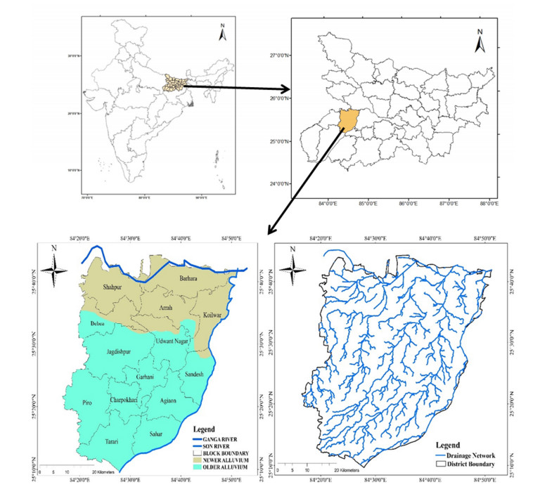
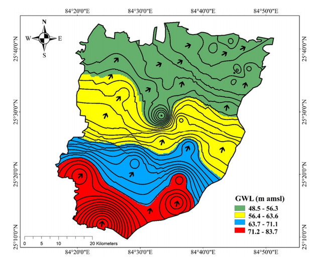
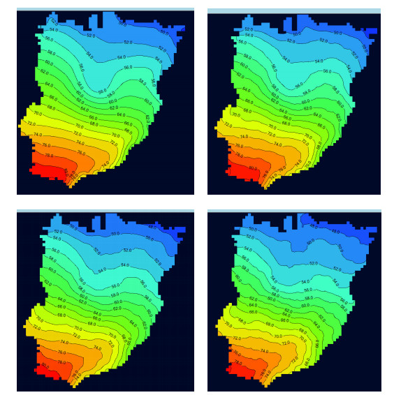
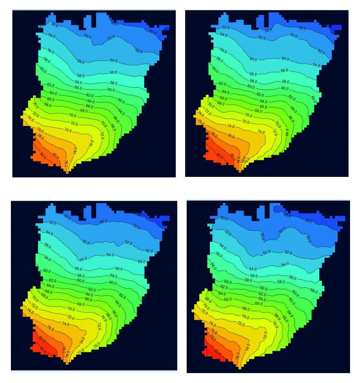
Water resources in India's Indo-Gangetic plains are over-exploited and vulnerable to impacts of climate change. The unequal spatial and temporal variation of meteorological, hydrological and hydrogeological parameters has created additional challenges for field engineers and policy planners. The groundwater and surface water are extensively utilized in the middle Gangetic plain for agriculture. The primary purpose of this study is to understand the discharge and recharge processes of groundwater system using trend analysis, and surface water and groundwater interaction using groundwater modelling. A comprehensive hydrological, and hydrogeological data analysis was carried out and a numerical groundwater model was developed for Bhojpur district, Bihar, India covering 2395 km² geographical area, located in central Ganga basin. The groundwater level data analyses for the year 2018 revealed that depth to water level varies from 3.0 to 9.0 meter below ground level (m bgl) in the study area. The M-K test showed no significant declining trend in the groundwater level in the study area. The groundwater modelling results revealed that groundwater head is higher in the southern part of the district and the groundwater flow direction is from south-west to north-east. The groundwater head fluctuation between the monsoon and the summer seasons was observed to be 2 m, it is also witnessed that groundwater is contributing more to rivers in the monsoon season in comparison with other seasons. Impact of reduction in pumping on groundwater heads was also investigated, considering a 10% reduction in groundwater withdrawal. The results indicated an overall head rise of 2 m in the southern part and 0.2–0.5 m in the middle and northern part of the district.

Keywords:

Citation: Sumant Kumar, Anuj Kumar Dwivedi, Chandra Shekhar Prasad Ojha, Vinod Kumar, Apourv Pant, P. K. Mishra, Nitesh Patidar, Surjeet Singh, Archana Sarkar, Sreekanth Janardhanan, C. P. Kumar, Mohammed Mainuddin. Numerical groundwater modelling for studying surface water-groundwater interaction and impact of reduced draft on groundwater resources in central Ganga basin[J]. Mathematical Biosciences and Engineering, 2022, 19(11): 11114-11136. doi: 10.3934/mbe.2022518

Related Papers:

[1]	Wei Zhang, Pengcheng Li, Donghe Pei . Circular evolutes and involutes of spacelike framed curves and their duality relations in Minkowski 3-space. AIMS Mathematics, 2024, 9(3): 5688-5707. doi: 10.3934/math.2024276
[2]	Emad Solouma, Ibrahim Al-Dayel, Meraj Ali Khan, Youssef A. A. Lazer . Characterization of imbricate-ruled surfaces via rotation-minimizing Darboux frame in Minkowski 3-space $\mathrm{E}_1^3$ . AIMS Mathematics, 2024, 9(5): 13028-13042. doi: 10.3934/math.2024635
[3]	Ayman Elsharkawy, Clemente Cesarano, Abdelrhman Tawfiq, Abdul Aziz Ismail . The non-linear Schrödinger equation associated with the soliton surfaces in Minkowski 3-space. AIMS Mathematics, 2022, 7(10): 17879-17893. doi: 10.3934/math.2022985
[4]	Kemal Eren, Soley Ersoy, Mohammad Nazrul Islam Khan . Simultaneous characterizations of alternative partner-ruled surfaces. AIMS Mathematics, 2025, 10(4): 8891-8906. doi: 10.3934/math.2025407
[5]	Chang Sun, Kaixin Yao, Donghe Pei . Special non-lightlike ruled surfaces in Minkowski 3-space. AIMS Mathematics, 2023, 8(11): 26600-26613. doi: 10.3934/math.20231360
[6]	Emad Solouma, Mohamed Abdelkawy . Family of ruled surfaces generated by equiform Bishop spherical image in Minkowski 3-space. AIMS Mathematics, 2023, 8(2): 4372-4389. doi: 10.3934/math.2023218
[7]	Kemal Eren, Hidayet Huda Kosal . Evolution of space curves and the special ruled surfaces with modified orthogonal frame. AIMS Mathematics, 2020, 5(3): 2027-2039. doi: 10.3934/math.2020134
[8]	Cai-Yun Li, Chun-Gang Zhu . Construction of the spacelike constant angle surface family in Minkowski 3-space. AIMS Mathematics, 2020, 5(6): 6341-6354. doi: 10.3934/math.2020408
[9]	Yanlin Li, Kemal Eren, Soley Ersoy . On simultaneous characterizations of partner-ruled surfaces in Minkowski 3-space. AIMS Mathematics, 2023, 8(9): 22256-22273. doi: 10.3934/math.20231135
[10]	Samah Gaber, Abeer Al Elaiw . Evolution of null Cartan and pseudo null curves via the Bishop frame in Minkowski space $\mathbb{R}^{2, 1}$ . AIMS Mathematics, 2025, 10(2): 3691-3709. doi: 10.3934/math.2025171

Abstract

1. Introduction

The investigation of surfaces and alternative frames in Lorentz–Minkowski space offers insights into the interplay between differential geometry and special relativity ^[1,2,3,4].

Ruled surfaces are surfaces that can be generated by moving a straight line in space according to specific rules. These surfaces have applications in various fields, including architecture, computer graphics, and differential geometry itself. While ruled surfaces are often studied in Euclidean or Riemannian geometries, examining them in the context of $E_{1}^{3}$ opens new perspectives and challenges due to the Lorentzian nature of spacetime. The use of alternative frames in differential geometry ^[5,6] provides a basis for understanding the geometric and physical properties of spacetime. This approach, extensively discussed in Wald's textbook ^[7], allows for the decomposition of the metric tensor into components corresponding to different types of vectors in the frame. Alternative frames have proven valuable in studying the kinematics of particles and observers in curved spacetimes, enabling the interpretation of relativistic effects and gravitational interactions. Furthermore, in the fields of partial differential equations, geometric analysis, mathematical physics, etc., soliton theory is a critical theory that attracts the attention of many researchers ^[8,9,10,11]. There are many applications of solitons in applied mathematics and pure mathematics, especially in partial differential equations, ordinary partial differential equations, Lie algebras, Lie groups, differential geometry, and algebraic geometry ^{[12,13,14,15]}. In ^[16], Manukure and Booker presented an overview of solitons and applications; they stated the research history of solitons and showed further developments. The paper ^[16] shows that solitons appear in various fields, particularly in physical contexts, including fluid dynamics, optical fibers, and quantum field theory. In each case, they are described by specific evolution equations that capture the relevant physics ^[17]. This work aims to explore the evolution of different types of timelike ruled surfaces using alternative frames in Minkowski space. By investigating the interplay between these surfaces and alternative frames, we enhance our understanding of the geometric structures of these surfaces in Lorentz-Minkowski 3-space.

This paper is organized as follows: In Section 2, we provide a brief overview of curves and timelike ruled surfaces and explore the relationship between these surfaces and alternative frames in Lorentz–Minkowski 3-space. Section 3 presents evolution equations for a given timelike curve and some timelike ruled surfaces generated by the alternative frame vectors of their associated timelike curves in Lorentz–Minkowski 3-space. Illustrated examples to support our main results are provided in Section 4, and we conclude with a summary of our findings in Section 5.

2. Geometric concepts

2.1. An alternative frame

Lorentz–Minkowski 3-space $E_{1}^{3}$ is the real vector space $E^{3}$ augmented by the Lorentzian inner product

$\begin{equation} \langle \mathbf{a}, \mathbf{b} \rangle_{E_{1}^{3}} = -a_{1}b_{1} + a_{2}b_{2} + a_{3}b_{3}, \end{equation}$

(2.1)

where $\mathbf{a} = (a_{1}, a_{2}, a_{3})$ and $\mathbf{b} = (b_{1}, b_{2}, b_{3}) \in E_{1}^{3}$ . The norm of $\mathbf{b}$ is $\|\mathbf{b}\| = \sqrt{ \langle \mathbf{b}, \mathbf{b} \rangle_{E_{1}^{3}}}$ .

The cross product of $\mathbf{a}$ and $\mathbf{b}$ is given by

$\begin{equation} \mathbf{a} \wedge_{E_{1}^{3}} \mathbf{b} = \langle -a_{3}b_{2} + a_{2}b_{3}, -a_{3}b_{1} + a_{1}b_{3}, a_{1}b_{2} - a_{2}b_{1} \rangle. \end{equation}$

(2.2)

If $\mathbf{r}(s): I \subseteq \mathbb{R} \longrightarrow E_{1}^{3}$ is a regular curve described by

$\begin{equation} \mathbf{r}(s) = (y(s), z(s), w(s)), \end{equation}$

(2.3)

where $I$ is an open interval and $y(s), z(s)$ , and $w(s) \in C^{3}$ , then $\mathbf{r}$ is spacelike if $\langle \mathbf{r}^{\prime}(s), \mathbf{r} ^{\prime}(s) \rangle_{E_{1}^{3}} > 0$ , timelike if $\langle \mathbf{r} ^{\prime}(s), \mathbf{r}^{\prime}(s) \rangle_{E_{1}^{3}} < 0$ , and lightlike if $\langle \mathbf{r}^{\prime}(s), \mathbf{r}^{\prime}(s) \rangle_{E_{1}^{3}} = 0$ , for all $s \in I$ .

The derivatives of the Frenet frame vectors of $\mathbf{r}(s)$ , which has tangent $\mathbf{T}(s)$ , principal normal $\mathbf{n}(s)$ , and binormal $\mathbf{p}(s)$ , take the form:

$\begin{equation} \frac{\partial }{\partial s} \begin{pmatrix} \mathbf{T}(s) \\ \mathbf{n}(s) \\ \mathbf{p}(s) \end{pmatrix} = \begin{pmatrix} 0 & \kappa (s) & 0 \\ \epsilon _{\mathbf{p}}\kappa (s) & 0 & \tau (s) \\ 0 & \epsilon _{\mathbf{T}}\tau (s) & 0 \end{pmatrix} \begin{pmatrix} \mathbf{T}(s) \\ \mathbf{n}(s) \\ \mathbf{p}(s) \end{pmatrix} , \end{equation}$

(2.4)

where

$\begin{equation} \langle \mathbf{T},\mathbf{T}\rangle _{E_{1}^{3}} = \epsilon _{\mathbf{T} },\quad \langle \mathbf{n},\mathbf{n}\rangle _{E_{1}^{3}} = \epsilon _{\mathbf{ n}},\quad \text{and}\quad \langle \mathbf{p},\mathbf{p}\rangle _{E_{1}^{3}} = -\epsilon _{\mathbf{T}}\epsilon _{\mathbf{n}} = \epsilon _{ \mathbf{p}}, \end{equation}$

(2.5)

and

$\begin{equation} \mathbf{T}\times _{E_{1}^{3}}\mathbf{n} = \mathbf{p},\quad \mathbf{n}\times _{E_{1}^{3}}\mathbf{p} = -\epsilon _{\mathbf{n}}\mathbf{T},\quad \text{and} \quad \mathbf{p}\times _{E_{1}^{3}}\mathbf{T} = -\epsilon _{\mathbf{T}}\mathbf{ n}. \end{equation}$

(2.6)

The functions $\kappa(s)$ and $\tau(s)$ represent the curvature and the torsion of the curve, respectively. For more details, see ^[2]. Additionally, this frame satisfies the following conditions:

$\begin{equation*} \mathbf{T}(s) = \frac{d\mathbf{r}/ds}{||d\mathbf{r}/ds||},\quad \mathbf{n}(s) = \frac{\mathbf{T}_{s}(s)}{||\mathbf{T}_{s}(s)||},\quad \mathbf{p}(s) = \mathbf{T }(s)\wedge _{E_{1}^{3}}\mathbf{n}(s), \end{equation*}$

where $\mathbf{T}_{s}(s) = d\mathbf{T}(s)/ds$ .

In this context, the time evolution equations for the given curve are written as follows:

$\begin{equation} \frac{\partial }{\partial t}\left( \begin{array}{c} \mathbf{T} \\ \mathbf{n} \\ \mathbf{p} \end{array} \right) = \left( \begin{array}{ccc} 0 & \alpha & \beta \\ \alpha & 0 & \gamma \\ \beta & -\gamma & 0 \end{array} \right) \left( \begin{array}{c} \mathbf{T} \\ \mathbf{n} \\ \mathbf{p} \end{array} \right) , \notag \label{eq:320} \end{equation}$

where $\alpha$ , $\beta$ , and $\gamma$ are the velocities of the curve, dependent on its curvatures.

Next, we explore the alternative frame of $\mathbf{r}(s)$ as a timelike curve in Lorentz–Minkowski 3-space. By examining this frame, we gain insights into the geometric properties and physical aspects of the curve, offering a fresh perspective on its behavior within the context of differential geometry.

Consider $\mathbf{r} = \mathbf{r}(s)$ as a given timelike curve with arc length parameter $s$ in $E_{1}^{3}$ . Let $\{\mathbf{T}(s), \mathbf{n}(s), \mathbf{p}(s)\}$ and $\{\mathbf{n}(s), \mathbf{C}(s), \mathbf{W}(s)\}$ be the Frenet frame and the alternative frame of $\mathbf{r}$ , respectively. The alternative frame can then be defined as follows:

$\begin{eqnarray} \mathbf{C}(s) & = &\frac{\mathbf{n}^{\prime }(s)}{||\mathbf{n}^{\prime }(s)||}, \\ \ \mathbf{W}(s) & = &\frac{\tau (s)}{\sqrt{|\kappa ^{2}(s)-\tau ^{2}(s)|}} \mathbf{T}(s)+\frac{\kappa (s)}{\sqrt{|\kappa ^{2}(s)-\tau ^{2}(s)|}}(s) \mathbf{p}(s), \end{eqnarray}$

(2.7)

where $\mathbf{n}$ , $\mathbf{C}$ , and $\mathbf{W}$ represent the spacelike normal, the timelike derivative of the normal, and the spacelike Darboux vector of $\mathbf{r}(s)$ , respectively ^[5]. Clearly, the Darboux vector $\mathbf{W}$ is orthogonal to the normal vector $\mathbf{n}(s)$ ^[6,18].

The derivative formulas for the alternative frame of $\mathbf{r}(s)$ can be expressed as follows:

$\begin{equation} \frac{\partial}{\partial s} \begin{pmatrix} \mathbf{n}(s) \\ \mathbf{C}(s) \\ \mathbf{W}(s) \end{pmatrix} = \begin{pmatrix} 0 & \sigma(s) & 0 \\ \sigma(s) & 0 & \varrho(s) \\ 0 & \varrho(s) & 0 \end{pmatrix} \begin{pmatrix} \mathbf{n}(s) \\ \mathbf{C}(s) \\ \mathbf{W}(s) \end{pmatrix} , \end{equation}$

(2.8)

where

$\begin{equation} \sigma (s) = \sqrt{|\kappa ^{2}(s)-\tau ^{2}(s)|},\quad \varrho (s) = \frac{ \kappa ^{2}(s)(\frac{\tau (s)}{\kappa (s)})^{\prime }}{\kappa ^{2}(s)-\tau ^{2}(s)}, \end{equation}$

(2.9)

are differentiable functions referred to as alternative curvatures that depend on the curvatures of $\mathbf{r}(s)$ .

Since the principal normal vector $\mathbf{n}(s)$ is common to both frames, the relationship between the two frames can be expressed in matrix form as ^[5]:

$\begin{equation} \left( \begin{array}{c} \mathbf{T} \\ \mathbf{n} \\ \mathbf{p} \end{array} \right) = \left( \begin{array}{ccc} 0 & \frac{\kappa (s)}{\sqrt{|\kappa ^{2}(s)-\tau ^{2}(s)|}} & -\frac{\tau (s) }{\sqrt{|\kappa ^{2}(s)-\tau ^{2}(s)|}} \\ 1 & 0 & 0 \\ 0 & -\frac{\tau (s)}{\sqrt{|\kappa ^{2}(s)-\tau ^{2}(s)|}} & \frac{\kappa (s) }{\sqrt{|\kappa ^{2}(s)-\tau ^{2}(s)|}} \end{array} \right) \left( \begin{array}{c} \mathbf{n} \\ \mathbf{C} \\ \mathbf{W} \end{array} \right), \end{equation}$

(2.10)

$\begin{equation} \left( \begin{array}{c} \mathbf{n} \\ \mathbf{C} \\ \mathbf{W} \end{array} \right) = \left( \begin{array}{ccc} 0 & 1 & 0 \\ \frac{\kappa (s)}{\sqrt{|\kappa ^{2}(s)-\tau ^{2}(s)|}} & 0 & -\frac{\tau (s) }{\sqrt{|\kappa ^{2}(s)-\tau ^{2}(s)|}} \\ -\frac{\tau (s)}{\sqrt{|\kappa ^{2}(s)-\tau ^{2}(s)|}} & 0 & \frac{\kappa (s) }{\sqrt{|\kappa ^{2}(s)-\tau ^{2}(s)|}} \end{array} \right) \left( \begin{array}{c} \mathbf{T} \\ \mathbf{n} \\ \mathbf{p} \end{array} \right) . \end{equation}$

(2.11)

Considering that

$\begin{equation} \mathbf{n} \times_{E_{1}^{3}} \mathbf{C} = \mathbf{W}, \quad \mathbf{C} \times_{E_{1}^{3}} \mathbf{W} = \mathbf{n}, \quad \text{and} \quad \mathbf{n} \times_{E_{1}^{3}} \mathbf{W} = \mathbf{C}, \end{equation}$

(2.12)

and to simplify the form of our equations, we will use the following symbols:

$\begin{equation*} \digamma_{1} = \frac{\kappa(s)}{\sqrt{|\kappa^2(s) - \tau^2(s)|}}, \quad \digamma_{2} = \frac{\tau(s)}{\sqrt{|\kappa^2(s) - \tau^2(s)|}}. \end{equation*}$

The equations of motion for the alternative frame $\{\mathbf{n}(s), \mathbf{C }(s), \mathbf{W}(s)\}$ of $\mathbf{r}(s)$ can be expressed broadly, similar to Eq (2.8) as ^[19]:

$\begin{equation} \frac{\partial}{\partial t} \begin{pmatrix} \mathbf{n}(s) \\ \mathbf{C}(s) \\ \mathbf{W}(s) \end{pmatrix} = \begin{pmatrix} 0 & \delta(s) & \theta(s) \\ \delta(s) & 0 & \phi(s) \\ - \theta & \phi(s) & 0 \end{pmatrix} \begin{pmatrix} \mathbf{n}(s) \\ \mathbf{C}(s) \\ \mathbf{W}(s) \end{pmatrix} , \end{equation}$

(2.13)

where $\delta$ , $\theta$ , and $\phi$ represent the alternative velocities of the aforementioned curve.

The alternative frame provides a distinct basis for analyzing the geometry of curves and surfaces. The vectors in this alternative frame often offer insights into various geometric properties and can simplify the analysis of complex structures ^[20]. In ^[21], a novel class of ruled surface known as the $\mathbf{C}$ -ruled surface is introduced, defined through the alternative frame associated with a base curve. The differential geometric properties of this surface are examined, including the striction line, distribution parameter, fundamental forms, as well as Gaussian and mean curvatures. In our work, we will examine the evolution equations for specific types of ruled surfaces with significant geometric applications. By employing the alternative frame associated with the basic curve of these surfaces, we will investigate their key geometric properties. This comprehensive analysis will provide deeper insights into the dynamics of the local curvatures during their evolution. Our work aims to advance the understanding of surface behavior in Lorentz–Minkowski 3-space, with implications across various disciplines.

2.2. Ruled surfaces in Minkowski space

A ruled surface is one generated by moving a straight line, known as the ruling line, according to specific rules. Each ruling line lies entirely on the surface, forming a family of lines that cover the surface. Mathematically, a ruled surface can be defined as follows (see ^[3,22,23,24] for more details):

$\begin{equation} \mathbb{S}(s,v) = \mathbf{r}(s)+v\,\Phi (s)\,|\,s\in I,v\in J, \end{equation}$

(2.14)

where $\mathbf{r}(s)$ is the base curve of $\mathbb{S}(s, v)$ in Lorentz–Minkowski 3-space, $v$ is a function defined on an interval $J$ , and $\Phi$ is a fixed vector representing the direction of the ruling lines. The choice of the curve $\mathbf{r}(s)$ and the function $v$ determines the specific properties and shape of the ruled surface.

Definition 2.1. A surface in Lorentz–Minkowski 3-space is classified as spacelike or timelike based on the nature of the induced metric at the surface: a positive definite Riemannian metric corresponds to a spacelike surface, while a negative definite Riemannian metric corresponds to a timelike surface. Alternatively, a spacelike surface has a normal vector that is timelike, whereas a timelike surface has a normal vector that is spacelike^[25].

For the ruled surface defined by Eq (2.14), the normal vector at a point is defined as a vector perpendicular to the tangent plane of the surface at that point. This normal vector is crucial for defining the geometry of the surface and is denoted by

$\begin{equation} \mathbf{N} = \frac{\mathbb{S}_{s}\times \mathbb{S}_{v}}{||\mathbb{S}_{s}\times \mathbb{S}_{v}||}. \end{equation}$

(2.15)

The first and second fundamental forms on the surface $\mathbb{S}$ , along with their quantities, are respectively expressed by

$\begin{equation} I = \langle d\mathbb{S},d\mathbb{S}\rangle = Eds^{2}+2\,Fdsdv+Gdv^{2}, \end{equation}$

(2.16)

where,

$\begin{equation*} E = \langle \mathbb{S}_{s},\mathbb{S}_{s}\rangle ,\,F = \langle \mathbb{S}_{s}, \mathbb{S}_{v}\rangle = \langle \mathbb{S}_{v},\mathbb{S}_{s}\rangle ,\,G = \langle \mathbb{S}_{v},\mathbb{S}_{v}\rangle , \end{equation*}$

and

$\begin{equation} II = \langle d\mathbb{S},\mathbf{N}\rangle = eds^{2}+2fdsdv+gdv^{2}, \end{equation}$

(2.17)

noting that

$\begin{equation*} e = \langle \mathbb{S}_{ss},\mathbf{N}\rangle ,\,f = \langle \mathbb{S}_{sv}, \mathbf{N}\rangle = \langle \mathbb{S}_{vs},\mathbf{N}\rangle ,\,g = \langle \mathbb{S}_{vv},\mathbf{N}\rangle . \end{equation*}$

The Gaussian and mean curvatures of $\mathbb{S}$ play a vital role in characterizing the shape and properties of $\mathbb{S}$ . They are given by the following forms:

$\begin{equation} K = \epsilon _{\mathbf{N}}\frac{{eg-f^{2}}}{{EG-F^{2}}} = \frac{Det(h)}{ Det(\Delta )};\epsilon _{\mathbf{N}} = \mathbf{\langle N},\mathbf{N\rangle ,} \end{equation}$

(2.18)

and

$\begin{equation} H = \frac{\epsilon _{\mathbf{N}}}{2}\,\frac{eG-2fF+gE}{\left( EG-F^{2}\right) } = \frac{1}{2}\epsilon _{\mathbf{N}}tr(h^{\ast }\Delta ), \end{equation}$

(2.19)

where $\Delta = EG-F^{2}$ , $h = eg-f^{2}$ , and $h^{\ast }$ denotes the inverse matrix of $h\$ ^[25].

It is worth noting that, as stated in ^[26], the surface evolution denoted by $\mathbb{S}(s, v, t)$ and its corresponding flow $\frac{\partial \mathbb{S} (s, v, t)}{\partial t}$ are considered inextensible if the following condition is satisfied:

$\begin{equation} \begin{cases} \frac{\partial E}{\partial t} = 0, \\ \frac{\partial F}{\partial t} = 0, \\ \frac{\partial G}{\partial t} = 0. \end{cases} \end{equation}$

(2.20)

3. Evolution equations and alternative frame

In this section, we focus on deriving the evolution equations for special types of ruled surfaces using an alternative frame for their curves. To achieve this, we first derive the evolution equations for a timelike curve, highlighting its unique geometric properties and implications within differential geometry. The main result of this analysis is presented in the following theorem.

Theorem 3.1. Let $\mathbf{r} = \mathbf{r}(s, t)$ be a given timelike curve which has the alternative frame $\{\mathbf{n}, \mathbf{C}, \mathbf{W}\}$ in $E_{1}^{3}$ , then the evolution equations of the alternative curvatures of $\mathbf{r}$ can be described as:

$\begin{equation} \begin{cases} \sigma _{t} = \delta _{s}+\varrho \,\theta , \\ \varrho _{t} = \phi _{s}-\sigma \,\theta , \end{cases} \end{equation}$

(3.1)

where $\delta,$ $\phi$ and $\theta$ are the velocities of $\mathbf{r}$ .

Proof. Let us write Eq (2.8) in a simple form as

$\begin{equation} \frac{\partial \mathbf{A}}{\partial s} = \mathbf{L}\,\mathbf{A}, \end{equation}$

(3.2)

where

$\begin{equation*} \mathbf{A} = \left( \begin{array}{c} \mathbf{n} \\ \mathbf{C} \\ \mathbf{W} \end{array} \right) ,\quad \mathbf{L} = \begin{pmatrix} 0 & \sigma (s) & 0 \\ \sigma (s) & 0 & \varrho (s) \\ 0 & \varrho (s) & 0 \end{pmatrix} . \end{equation*}$

Similar to that procedure, Eq (2.13) can be reformulated as

$\begin{equation} \frac{\partial\mathbf{A}}{\partial t} = \mathbf{M}\,\mathbf{A}, \end{equation}$

(3.3)

where

$\begin{equation*} \mathbf{M} = \begin{pmatrix} 0 & \delta(s) & \theta(s) \\ \delta(s) & 0 & \phi(s) \\ - \theta & \phi(s) & 0 \end{pmatrix} . \end{equation*}$

From this point, by applying the compatibility conditions $\frac{\partial}{ \partial s}\frac{\partial \mathbf{A}}{\partial t} = \frac{\partial}{\partial t }\frac{\partial \mathbf{A}}{\partial s}$ and making some calculations, one can obtain

$\begin{equation} \frac{\partial \mathbf{L}}{\partial t} - \frac{\partial \mathbf{M}}{\partial s} + [ \mathbf{L}, \mathbf{M}] = 0_{3\times 3}, \end{equation}$

(3.4)

with Lie bracket $[ \mathbf{L}, \mathbf{M}] = \mathbf{L} \mathbf{M} - \mathbf{M} \mathbf{L}$ .

We conclude from Eq (3.4), after simple calculations, we obtain the following system of equations

$\begin{equation*} \begin{cases} \sigma_{t} - \delta_s - \varrho\, \theta = 0, \\ \varrho_{t} - \phi_s + \sigma\, \theta = 0, \\ \theta_s - \sigma\, \phi + \varrho\, \delta = 0, \end{cases} \end{equation*}$

which leads to the completeness of the proof. □

Our focus now shifts to deriving evolution equations for specific ruled surfaces generated by the alternative frame vectors associated with their curves. This will be addressed through the following theorems.

Theorem 3.2. Consider $\mathbf{r} = \mathbf{r}(s, t)$ is a timelike curve that has the alternative frame $\{\mathbf{n}, \mathbf{C}, \mathbf{W} \}$ in Lorentz–Minkowski 3-space. Let $\mathbb{S}_\mathbf{n}$ be a timelike $\mathbf{n}$ -ruled surface whose $\mathbf{r}$ is its base curve, then the following are hold:

1) The evolution equation of $\mathbb{S}_{\mathbf{n}}$ is

$\begin{equation} \digamma _{2}\frac{\partial \digamma _{2}}{\partial t}-\left( \digamma _{1}+v\sigma \right) \frac{\partial \digamma _{1}}{\partial t} = 0. \end{equation}$

(3.5)

2) $\mathbb{S}_{\mathbf{n}}$ is minimal surface if and only if

$\begin{equation*} \digamma _{2}\tau _{2}-\left( \digamma _{1}+v\tau _{1}\right) _{s} = 0. \end{equation*}$

3) $\mathbb{S}_{\mathbf{n}}$ is developable if and only if

$\begin{equation*} \left( \digamma _{1}+v\sigma \right) -\digamma _{2}\varrho = 0. \end{equation*}$

Proof. Since, the ruled surface $\mathbb{S}_{\mathbf{n}}$ can be written as:

$\begin{equation} \mathbb{S}_{\mathbf{n}}(s,v,t) = \mathbf{r}(s,t)+v\,\mathbf{n}(s,t), \end{equation}$

(3.6)

then by differentiating this equation, we get

$\begin{equation*} \begin{cases} \left( \mathbb{S}_{\mathbf{n}}\right) _{s} = \left( \digamma _{1}+v\sigma \right) \mathbf{C}-\varrho \mathbf{W}, \\ \left( \mathbb{S}_{\mathbf{n}}\right) _{v} = \mathbf{n}. \end{cases} \end{equation*}$

From Eq (2.15), the normal on $\mathbf{N}$ is obtained:

$\begin{equation} \mathbf{N} = \frac{1}{\sqrt{-\frac{\tau ^{2}}{\kappa ^{2}(s)-\tau ^{2}(s)} +\left( \digamma _{1}+v\sigma \right) ^{2}}}\left( 0,\digamma _{2},-\digamma _{1}-v\sigma \right). \end{equation}$

(3.7)

In the light of the above, the first fundamental quantities are

$\begin{equation} E = \digamma _{2}^{2}-\left( \digamma _{1}+v\sigma \right) ^{2},\,\,\,\,\,F = 0,\,\,\,\,\,G = 1, \end{equation}$

(3.8)

which lead to

$\begin{equation} I = EG-F^{2} = \digamma _{2}^{2}-\left( \digamma _{1}+v\sigma \right) ^{2}. \end{equation}$

(3.9)

The second derivatives of Eq (3.6) with respect to $s$ and $v$ are expressed as

$\begin{equation*} \begin{cases} \left( \mathbb{S}_{\mathbf{n}}\right) _{ss} = \sigma \left( \digamma _{1}+v\sigma \right) \mathbf{n}+\left( \left( \digamma _{1}+v\sigma \right) _{s}-\digamma _{2}\varrho \right) \mathbf{C} \\ +\left( \varrho \left( \digamma _{1}+v\sigma \right) -\left( \digamma _{2}\right) _{s}\right) \mathbf{W}, \\ \left( \mathbb{S}_{\mathbf{n}}\right) _{vv} = 0, \\ \left( \mathbb{S}_{\mathbf{n}}\right) _{vs} = \left( \mathbb{S}_{\mathbf{n} }\right) _{sv} = \sigma \mathbf{C}. \end{cases} \end{equation*}$

From this, the second fundamental form is given as follows:

$\begin{eqnarray} II & = &eg-f^{2} \\ & = &-\left( \frac{\sigma ^{2}\left( \left( \digamma _{1}+v\sigma \right) -\digamma _{2}\varrho \right) ^{2}}{\left( \digamma _{1}+v\sigma \right) ^{2}-\digamma _{2}^{2}}\right) , \end{eqnarray}$

(3.10)

where,

$\begin{equation} \begin{cases} e = \mathbf{\langle }\left( \mathbb{S}_{\mathbf{n}}\right) _{ss},\mathbf{ N\rangle } = \frac{_{\digamma _{2}^{2}\varrho -\digamma _{2}\left( \digamma _{1}+v\sigma \right) _{s}}}{\sqrt{(\digamma _{1}+v\sigma )^{2}-\digamma _{2}^{2}}}, \\ f = \mathbf{\langle }\left( \mathbb{S}_{\mathbf{n}}\right) _{sv},\mathbf{ N\rangle } = \mathbf{\langle }\left( \mathbb{S}_{\mathbf{n}}\right) _{vs}, \mathbf{N\rangle } = \frac{\sigma \left( \left( \digamma _{1}+v\sigma \right) -\digamma _{2}\varrho \right) }{\sqrt{\left( \digamma _{1}+v\sigma \right) ^{2}-\digamma _{2}^{2}}}, \\ g = \mathbf{\langle }\left( \mathbb{S}_{\mathbf{n}}\right) _{vv},\mathbf{ N\rangle } = 0. \end{cases} \end{equation}$

(3.11)

From the aforementioned data, the Gaussian and mean curvatures for the surface $\mathbb{S}_{n}$ are given as follows:

$\begin{equation} \begin{cases} K = \left( \frac{\sigma (\left( \digamma _{1}+v\sigma \right) -\digamma _{2}\varrho )}{\sqrt{-\digamma _{2}^{2}+\left( \digamma _{1}+v\sigma \right) ^{2}}}\right) ^{2}, \\ H = \frac{-1}{2}\left( \frac{_{\digamma _{2}^{2}\varrho -\digamma _{2}\left( \digamma _{1}+v\sigma \right) _{s}}}{(-\digamma _{2}^{2}+\left( \digamma _{1}+v\sigma \right) ^{\frac{3}{2}}}\right) , \end{cases} \end{equation}$

(3.12)

therefore, the surface $\mathbb{S}_{n}$ is minimal if and only if

$\begin{equation*} -\digamma _{2}^{2}\varrho -\digamma _{2}\left( \digamma _{1}+v\sigma \right) _{s} = 0. \end{equation*}$

On the other hand, the surface $\mathbb{S}_{n}$ can be described as a developable if and only if

$\begin{equation*} \sigma ((\digamma _{1}+v\sigma)-\digamma _{2}\varrho ) = 0. \end{equation*}$

In light of the benefit of Eq (2.20), the evolution of the surface is obtained:

$\begin{equation*} \digamma _{2}\frac{\partial \digamma _{2}}{\partial t}-\left( \digamma _{1}+v\sigma \right) \frac{\partial \digamma _{1}}{\partial t} = 0. \end{equation*}$

This finishes the proof. □

Theorem 3.3. Assume that $\mathbb{S}_{\mathbf{C}}$ is a timelike $\mathbf{C}$ -ruled surface and $\mathbf{r}(s, t)$ be its timelike curve, which has the alternative frame vectors $\mathbf{n}, \mathbf{C}, \mathbf{W}$ in Lorentz–Minkowski 3-space. The surface $\mathbb{S}_{\mathbf{C}}$ satisfies the following:

1) It is minimal if and only if

$\begin{equation} \left( \begin{array}{c} v\sigma \left( -\digamma _{1}(\sigma -\varrho )-(v\sigma )_{s}+\left( \digamma _{1}\sigma +v\varrho \right) _{s}\right) \\ +\digamma _{2}\mathbf{(}\digamma _{1}\sigma +(v\sigma )_{s}\mathbf{)} +\digamma _{1}\sigma \mathbf{(}-\digamma _{2}+v(\sigma +\varrho )\mathbf{)} \end{array} \right) = 0 \end{equation}$

(3.13)

holds.

2) The surface is developable if and only if

$\begin{equation} v\sigma +v\varrho -\digamma _{2} = 0 \end{equation}$

(3.14)

is hold.

3) It has the evolution equation:

$\begin{equation} \digamma _{1}\frac{\partial \digamma _{1}}{\partial t}+(-\digamma _{2}+v\varrho )\frac{\partial \digamma _{2}}{ \partial t} = 0. \end{equation}$

(3.15)

Proof. The parametric representation of the $\mathbb{S}_{\mathbf{C}}$ surface can be formulated as

$\begin{equation} \mathbb{S}_{\mathbf{C}}(s,v,t) = \mathbf{r}(s,t)+v\mathbf{C}(s,t). \end{equation}$

(3.16)

The partial differentials of the surface $\mathbb{S}_{\mathbf{C}}$ with respect to $s$ and $v$ are given from

$\begin{equation*} \begin{cases} \left( \mathbb{S}_{\mathbf{C}}\right) _{s} = v\sigma \mathbf{n}+ \digamma _{1} \mathbf{C}+(-\digamma _{2}+v\varrho )\mathbf{W}, \\ \left( \mathbb{S}_{\mathbf{C}}\right) _{v} = \mathbf{C}. \end{cases} \end{equation*}$

Again, the surface differentials with respect to the parameters $s$ and $v$ are expressed as follows:

$\begin{equation*} \begin{cases} \left( \mathbb{S}_{\mathbf{C}}\right) _{ss} = \left( \sigma \digamma _{1}+(v\sigma )_{s}\right) \mathbf{n}, \\ +(v\sigma ^{2}+\left( \digamma _{1}\right) _{s}+\varrho (-\digamma _{2}+v\varrho ))\mathbf{C}+((-\digamma _{2}+v\varrho )_{s}+\digamma _{1}\varrho )\mathbf{W} \\ \left( \mathbb{S}_{\mathbf{C}}\right) _{vv} = 0, \\ \left( \mathbb{S}_{\mathbf{C}}\right) _{vs} = \left( \mathbb{S}_{\mathbf{C} }\right) _{sv} = \sigma \mathbf{n}+\varrho \mathbf{W}. \end{cases} \end{equation*}$

From this, the normal relative to the surface is given by

$\begin{equation} \mathbf{N} = \frac{1}{\sqrt{(v\sigma )^{2}+(-\digamma _{2}+v\varrho )^{2}}} (\digamma _{2}-v\sigma ,0,v\sigma ). \end{equation}$

(3.17)

In light of the above-mentioned data related to surface calculations, the first and second fundamental forms with their quantities are, respectively

$\begin{eqnarray} E & = &(v\sigma )^{2}-\digamma _{1}^{2}+(-\digamma _{2}+v\varrho )^{2}, \\ F & = &-\digamma _{1},\,\,\,\,\,G = -1, \end{eqnarray}$

(3.18)

which give us

$\begin{equation} I = -(v\sigma )^{2}-(-\digamma _{2}+v\varrho )^{2}, \end{equation}$

(3.19)

and,

$\begin{equation} \begin{cases} e = \frac{v\sigma (-\digamma _{1}(\sigma -\varrho )-(v\sigma )_{s}+\left( \digamma _{1}\sigma +v\varrho \right) _{s})+\digamma _{2}\left( \digamma _{1}\sigma +v\varrho \right) _{s})}{\sqrt{(v\sigma )^{2}+(-\digamma _{2}+v\varrho )^{2}}}, \\ f = \frac{-\sigma (-\digamma _{2}+v\sigma +v\varrho )}{\sqrt{(v\sigma )^{2}+(-\digamma _{2}+v\varrho )^{2}}}, \\ g = 0. \end{cases} \end{equation}$

(3.20)

From this, we have

$\begin{equation} II = \frac{\sigma ^{2}(-\digamma _{2}+v\sigma +v\varrho )^{2}}{(v\sigma )^{2}+(-\digamma _{2}+v\varrho )^{2}}. \end{equation}$

(3.21)

The geometric meanings of the surface $\mathbb{S}_{\mathbf{C}}$ are represented by its Gaussian and mean curvatures. They are given from

$\begin{equation} \begin{cases} K = -(\frac{\sigma (-\digamma _{2}+v\sigma +v\varrho )}{\sqrt{(v\sigma )^{2}+(-\digamma _{2}+v\varrho )^{2}}})^{2}, \\ H = \frac{-1}{2}\frac{v\sigma \mathbf{(}-\digamma _{1}(\sigma -\varrho )-(v\sigma )_{s}+(\digamma _{1}\sigma +v\varrho )_{s}\mathbf{)}+\digamma _{2} \mathbf{(}\digamma _{1}\sigma +(v\sigma )_{s}\mathbf{)}+\digamma _{1}\sigma \mathbf{(}-\digamma _{2}+v(\sigma +\varrho )\mathbf{)}}{((v\sigma )^{2}+(-\digamma _{2}+v\varrho )^{2})^{\frac{3}{2}}}. \end{cases} \end{equation}$

(3.22)

As a result of the above, the surface $\mathbb{S}_{\mathbf{C}}$ is minimal when

$\begin{equation*} \left( \begin{array}{c} v\sigma \mathbf{(}-\digamma _{1}(\sigma -\varrho )-(v\sigma )_{s}+(\digamma _{1}\sigma +v\varrho )_{s}\mathbf{)} \\ +\digamma _{2}\mathbf{(}\digamma _{1}\sigma +(v\sigma )_{s}\mathbf{)} +\digamma _{1}\sigma \mathbf{(}-\digamma _{2}+v(\sigma +\varrho )\mathbf{)} \end{array} \right) = 0 \end{equation*}$

holds.

Besides, the surface $\mathbb{S}_{\mathbf{C}}$ is classified as a developable whenever

$\begin{equation*} -\digamma _{2}+v\sigma +v\varrho = 0, \end{equation*}$

is hold.

By applying Eq (2.20), the evolution condition for this surface is expressed as

$\begin{equation*} \digamma _{1}\frac{\partial \digamma _{1}}{\partial t}+(-\digamma _{2}+v\varrho )\frac{\partial \digamma _{2}}{ \partial t} = 0. \end{equation*}$

Hence, the proof is completed. □

Theorem 3.4. Suppose that $\mathbb{S}_{\mathbf{W}}$ is a timelike $\mathbf{W}$ -ruled surface generated by the alternative vector $\mathbf{W}$ of its base curve $\mathbf{r}$ in Lorentz–Minkowski 3-space. Then, the following statements are satisfied:

1) $\mathbb{S}_\mathbf{W}$ is a developable surface.

2) It has the following evolution equation:

$\begin{equation} \digamma _{2}\frac{\partial \digamma _{2}}{\partial t}-\left( \digamma _{1}+v\varrho \right) \frac{\partial \digamma _{1}}{\partial t} = 0. \end{equation}$

(3.23)

Proof. Since the surface $\mathbb{S}_{\mathbf{W}}$ has the following parametric representation

$\begin{equation} \mathbb{S}_{\mathbf{W}}(s,v,t) = \mathbf{r}(s,t)+v\mathbf{W}(s,t), \end{equation}$

(3.24)

then by differentiating this equation twice with respect to $s$ and $v$ , we obtain the following

$\begin{equation*} \begin{cases} \left( \mathbb{S}_{\mathbf{W}}\right) _{s} = (\digamma _{1}+v\varrho )\mathbf{C }-\digamma _{2}\mathbf{W}, \\ \left( \mathbb{S}_{\mathbf{W}}\right) _{v} = \sigma \mathbf{W}, \\ \left( \mathbb{S}_{\mathbf{W}}\right) _{ss} = \sigma (\digamma _{1}+v\varrho ) \mathbf{n} \\ +\left( -\digamma _{2}\varrho +\left( \digamma _{1}+v\varrho \right) _{s}\right) \mathbf{C}+(\varrho (\digamma _{1}+v\varrho )-\left( \digamma _{2}\right) _{s})\mathbf{W}, \\ \left( \mathbb{S}_{\mathbf{W}}\right) _{vv} = 0, \\ \left( \mathbb{S}_{\mathbf{W}}\right) _{vs} = \left( \mathbb{S}_{\mathbf{W} }\right) _{sv} = \varrho \mathbf{C}. \end{cases} \end{equation*}$

From this, we have the normal

$\begin{equation} \mathbf{N} = (1,0,0), \end{equation}$

(3.25)

and

$\begin{equation} \begin{cases} E = \mathbf{\langle }\left( \mathbb{S}_{\mathbf{W}}\right) _{s},\left( \mathbb{ S}_{\mathbf{W}}\right) _{s}{\rangle } = -( \digamma _{1} +v\varrho )^{2}+\digamma _{2}^{2}, \\ F = \mathbf{\langle }\left( \mathbb{S}_{\mathbf{W}}\right) _{s},\left( \mathbb{ S}_{\mathbf{W}}\right) _{v}{\rangle } = -\digamma _{2}, \\ G = \mathbf{\langle }\left( \mathbb{S}_{\mathbf{W}}\right) _{v},\left( \mathbb{ S}_{\mathbf{W}}\right) _{v}{\rangle } = 1, \end{cases} \end{equation}$

(3.26)

$\begin{equation} I = -(\digamma _{1}+v\varrho )^{2}, \end{equation}$

(3.27)

and also

$\begin{equation} e = \mathbf{\langle }\left( \mathbb{S}_{\mathbf{W}}\right) _{ss},\mathbf{ N\rangle } = \sigma (\digamma _{1}+v\varrho ),\,\,\,\,\,f = \mathbf{\langle } \left( \mathbb{S}_{\mathbf{W}}\right) _{vs},\mathbf{N\rangle } = 0,\,\,\,\,\,g = \mathbf{\langle }\left( \mathbb{S}_{\mathbf{W}}\right) _{vv},\mathbf{ N\rangle } = 0, \end{equation}$

(3.28)

$\begin{equation} II = 0. \end{equation}$

(3.29)

Further, the Gaussian and mean curvatures of $\mathbb{S}_{\mathbf{W}}$ are calculated as

$\begin{equation} K = 0,\,\,\,\,\,H = \frac{-\sigma }{2\left( \digamma _{1}+v\varrho \right) }, \end{equation}$

(3.30)

As a consequence, this surface is developable and not minimal.

Under the previous data, the evolution equation for the surface $\mathbb{S}_{ \mathbf{W}}$ is given by

$\begin{equation*} \digamma _{2}\frac{\partial \digamma _{2}}{\partial t}-\left( \digamma _{1}+v\varrho \right) \frac{\partial \digamma _{1}}{\partial t} = 0. \end{equation*}$

Thus, the result is clear. □

4. Application

In this section, we are interested in providing a practical example to demonstrate the theoretical results that we obtained through our study of the three special ruled surfaces: $\mathbf{n}$ -ruled, $\mathbf{C}$ -ruled, and $\mathbf{W}$ -ruled surfaces.

Consider $\mathbf{r}(s, t)$ be a timelike curve given by (see Figure 1)

$\begin{equation} \mathbf{r}(s,t) = \left( t\ \sinh \sqrt{2}s,t\ \cosh \sqrt{2}s,t\ s\right) . \end{equation}$

(4.1)

Figure 1. The timelike curve

$\mathbf{r}$ .

DownLoad: Full-Size Img PowerPoint

The tangent $\mathbf{T}$ , the normal $\mathbf{n}$ and the binormal $\mathbf{p }$ of $\mathbf{r}$ are, respectively

$\begin{equation*} \begin{cases} \mathbf{T} = \left( \sqrt{2}\cosh \sqrt{2}s,\sqrt{2}\sinh \sqrt{2} s,1\right) , \\ \mathbf{n} = \left( \sinh \sqrt{2}s,-\cosh \sqrt{2}s,0\right) , \\ \mathbf{p} = \left( \cosh \sqrt{2}s,\sinh \sqrt{2}s,\sqrt{2}\right) . \label {eq:00043} \end{cases} \end{equation*}$

The curvature functions of the considered curve are

$\begin{equation*} \kappa = \frac{2}{t},\,\,\,\,\,\tau = \frac{-\sqrt{2}}{t}, \end{equation*}$

also, the alternative frame vectors $\mathbf{n}, \mathbf{C}, \mathbf{W}$ of $\mathbf{r}$ are given as follows:

$\begin{equation} \begin{cases} \mathbf{n} = \left( \sinh \sqrt{2}s,-\cosh \sqrt{2}s,0\right) , \\ \mathbf{C} = \left( \cosh \sqrt{2}s,\sinh \sqrt{2}s,0\right) , \\ \mathbf{W} = \left( 0,0,1\right) . \end{cases} \end{equation}$

(4.2)

From this, the alternative curvatures of $\mathbf{r}$ are calculated as

$\begin{equation*} \sigma = \frac{\sqrt{2}}{t},\quad \varrho = 0. \end{equation*}$

The $\mathbf{n}$ -ruled surface that has $\mathbf{r}$ as a base curve is expressed by the following representation (see Figure 2)

$\begin{equation} \mathbb{S}_{\mathbf{n}} = \left( { t\sinh }\left( \sqrt{2}s\right) +v { \sinh }\left( \sqrt{2}s\right) ,{ t\cosh }\left( \sqrt{2} s\right) -v{ \cosh }\left( \sqrt{2}s\right) ,{ t }s\right) , \end{equation}$

(4.3)

Figure 2. The evolved

$\mathbf{n}$ -ruled surface

$\mathbb{S}_{\mathbf{n}}$ of the curve

$\mathbf{r}$ .

DownLoad: Full-Size Img PowerPoint

which has the normal

$\begin{equation*} \mathbf{N} = \left( \begin{array}{c} -\frac{{ t\cosh }\left( \sqrt{2}s\right) }{\sqrt{2v\left( v+2{ t\cosh }\left( 2\sqrt{2}s\right) \right) +{ t }^{2}{ \cosh } \left( 4\sqrt{2}s\right) }}, \\ \frac{{ t\sinh }\left( \sqrt{2}s\right) }{\sqrt{2v\left( v+2{ t\cosh }\left( 2\sqrt{2}s\right) \right) +{ t }^{2}{ \cosh } \left( 4\sqrt{2}s\right) }}, \\ -\frac{v+{ t\cosh }\left( 2\sqrt{2}s\right) }{\sqrt{v^{2}+2{ t }v { \cosh }\left( 2\sqrt{2}s\right) +\frac{1}{2}{ t }^{2}{ \cosh }\left( 4\sqrt{2}s\right) }} \end{array} \right) . \end{equation*}$

The first and second fundamental coefficients of the surface can be calculated, respectively

$\begin{equation*} E = -{ t }^{2}-2v^{2}-4{ t }v{ \cosh }\left( 2\sqrt{2}s\right) ,\ F = -\sqrt{2}{ t\sinh }\left( 2\sqrt{2}s\right) ,G = 1, \end{equation*}$

and

$\begin{equation*} \begin{cases} e = \frac{2{ t }^{2}{ \sinh }\left( 2\sqrt{2}s\right) }{\sqrt{ 2v\left( v+2{ t\cosh }\left( 2\sqrt{2}s\right) \right) +{ t }^{2} { \cosh }\left( 4\sqrt{2}s\right) }}, \\ f = \frac{{ t }}{\sqrt{v^{2}+2{ t }v{ \cosh }\left( 2\sqrt{2} s\right) +\frac{1}{2}{ t }^{2}{ \cosh }\left( 4\sqrt{2}s\right) }} , \\ g = 0. \end{cases} \end{equation*}$

Also, the surface's curvatures are

$\begin{eqnarray} K & = &\frac{2{ t }^{2}}{\left( 2v^{2}+4{ t }v{ \cosh }\left( 2 \sqrt{2}s\right) +{ t }^{2}{ \cosh }\left( 4\sqrt{2}s\right) \right) ^{2}}, \\ \,\,\,\,\,H & = &\frac{{ t }^{2}\left( -2+{ t }^{2}+2v^{2}+4{ t }v{ \cosh }\left( 2\sqrt{2}s\right) \right) { \sinh }\left( 2 \sqrt{2}s\right) }{\left( 2v^{2}+4{ t }v{ \cosh }\left( 2\sqrt{2} s\right) +{ t }^{2}{ \cosh }\left( 4\sqrt{2}s\right) \right) ^{3/2}}. \end{eqnarray}$

(4.4)

Similarly, the ruled surface that is generated by the vector $\mathbf{C}$ of the alternative frame of $\mathbf{r}$ can be written as (see Figure 3)

$\begin{equation} \mathbb{S}_{\mathbf{C}} = \left( v{ \cosh }\left( \sqrt{2}s\right) + { t\sinh }\left( \sqrt{2}s\right) ,{ t\cosh }\left( \sqrt{2} s\right) +v{ \sinh }\left( \sqrt{2}s\right) ,{ t }s\right). \end{equation}$

(4.5)

Figure 3. The evolved

$\mathbf{C}$ -ruled surface

$\mathbb{S}_{\mathbf{C}}$ of the curve

$\mathbf{r}$ .

DownLoad: Full-Size Img PowerPoint

Straightforward calculations of the surface $\mathbb{S}_{\mathbf{C}}$ lead to

$\begin{equation*} \mathbf{N} = \left( \frac{{ t\sinh }\left( \sqrt{2}s\right) }{\sqrt{ { t }^{2}+2v^{2}}},\frac{{ t\cosh }\left( \sqrt{2}s\right) }{ \sqrt{{ t }^{2}+2v^{2}}},-\frac{v}{\sqrt{\frac{{ t }^{2}}{2}+v^{2}} }\right) , \end{equation*}$

and

$\begin{equation*} E = -\text{ t }^{2}+2v^{2},\,\,\,\,\,\ F = -\sqrt{2}\text{ t },\,\,\,\,\,G = -1, \end{equation*}$

$\begin{equation*} e = \frac{2\text{ t }^{2}}{\sqrt{\text{ t }^{2}+2v^{2}}},\,\,\,\,\,\ f = \frac{ \text{ t }}{\sqrt{\frac{\text{ t }^{2}}{2}+v^{2}}},\,\,\,\,\,g = 0. \end{equation*}$

The Gaussian and mean curvatures of $\mathbb{S}_{\mathbf{C}}$ are

$\begin{equation} K = \frac{2\text{ t }^{2}}{\left( \text{ t }^{2}+2v^{2}\right) ^{2}} ,\,\,\,\,\,H = \frac{\text{ t }^{2}\left( \text{ t }^{2}-2\left( 1+v^{2}\right) \right) }{\left( \text{ t }^{2}+2v^{2}\right) ^{3/2}}. \end{equation}$

(4.6)

In the light of these results, this surface is neither developable nor minimal.

Likewise, the parametric representation for the ruled surface $\mathbb{S}_{ \mathbf{W}}$ reads as (see Figure 4)

$\begin{equation} \mathbb{S}_{\mathbf{W}} = \left( { t\sinh }\left( \sqrt{2}s\right) , { t\cosh }\left( \sqrt{2}s\right) ,{ t }s+v\right). \end{equation}$

(4.7)

Figure 4. The evolved

$\mathbf{W}$ -ruled surface

$\mathbb{S}_{\mathbf{W}}$ of the curve

$\mathbf{r}$ .

DownLoad: Full-Size Img PowerPoint

Making some special calculations related to the considered surface, we get

$\begin{equation*} \mathbf{N} = \left( -{ \sinh }\left( \sqrt{2}s\right) ,-{ \cosh } \left( \sqrt{2}s\right) ,0\right) , \end{equation*}$

and

$\begin{equation*} E = -\text{ t }^{2},\,\,\,\,\,F = \text{ t },\,\,\,\,\,G = 1,\,\,\,\,\,e = -2\text{ t },\,\,\,\,\,f = 0,\,\text{and}\,\ g = 0. \end{equation*}$

The Gaussian and mean curvatures are

$\begin{equation*} K = 0,\,\,\,\,\,H = -\frac{\text{ t }}{2}, \end{equation*}$

which describe $\mathbb{S}_{\mathbf{C}}$ as developable and not minimal.

5. Conclusions

In the three-dimensional Lorentz–Minkowski 3-space $E_{1}^{3}$ , we examined the evolution equations for specific types of ruled surfaces that have significant geometric and physical applications. We employed the alternative frame associated with the basic curve of these surfaces and investigated their key geometric properties. Through a comprehensive analysis, we gained deeper insights into the dynamics of the local curvatures exhibited by these surfaces during their evolution. This work advanced the understanding of the dynamical behavior of surfaces in Lorentz–Minkowski 3-space, with potential implications across various disciplines. Finally, we discussed applications of our preliminary findings, which contribute significantly to the broader field of differential geometry. Looking forward, several avenues for future research emerge. Our findings could be applied to physical models involving particle trajectories or gravitational fields, potentially revealing how timelike ruled surfaces might be utilized in practical scenarios or theoretical frameworks. Further studies could explore alternative frames in more complex settings or for other types of surfaces beyond ruled ones, which might lead to a broader understanding of geometric structures in relativity. The study of solitons through their evolution equations provides crucial insights into a wide range of phenomena, contributing to advances in both theoretical and applied sciences. Solitons are special types of solutions to nonlinear partial differential equations that maintain their shape while propagating at constant velocity. They are often associated with topological solutions and are significant in various fields ^[16]. Here are some potential applications of evolution equations related to solitons (topological solutions): In the field of mathematical physics, the study of solitons is essential for understanding integrable systems, where the evolution equations are exactly solvable. This has applications in theoretical models and helps in the development of new mathematical techniques. Also, in plasma physics, the evolution equations used in solitons can describe stable wave packets in plasma, which helps in understanding space weather–phenomena and the behavior of high-energy plasmas. By expanding on these aspects, in future research, we will combine the results and methods in ^[25,26,27] to deepen our knowledge and uncover new applications of differential geometry in both theoretical and practical contexts.

Author contributions

Yanlin Li: Conceptualization, Methodology; M. Khalifa Saad: Validation, Formal analysis; H. S. Abdel-Aziz: Writing-review, Supervision, Validation; H. M. Serry: Methodology, Writing-original draft; F. M. El-Adawy: Validation, editing. All authors have read and approved the final version of the manuscript for publication.

Use of AI tools declaration

The authors declare they have not used Artificial Intelligence (AI) tools in the creation of this article.

Acknowledgments

The authors express gratitude to the reviewers and editors for their helpful comments and suggestions.

Conflict of interest

All authors declare no conflicts of interest in this paper.

References

[1]	R. Kumar, R. D. Singh, K. D. Sharma, Water resources of India, Curr. Sci., 89 (2005), 794–811. https://www.jstor.org/stable/24111024
[2]	M. K. Goyal, R. Y. Surampalli, Impact of climate change on water resources in India, J. Environ. Eng., 144 (2018), 04018054. https://doi.org/10.1061/(ASCE)EE.1943-7870.0001394 doi: 10.1061/(ASCE)EE.1943-7870.0001394
[3]	K. Rudra, Combating flood and erosion in the lower ganga plain in India: some unexplored issues, in Disaster Studies, (2020), 173–186. https://doi.org/10.1007/978-981-32-9339-7_9
[4]	T. Oki, S. Kanae, Global hydrological cycles and world water resources, Science, 313 (2006), 1068–1072. https://doi.org/10.1126/science.1128845 doi: 10.1126/science.1128845
[5]	C. K. Pawe, A. Saikia, Unplanned urban growth: land use/land cover change in the Guwahati Metropolitan Area, India, Geografisk Tidsskrift-Danish J. Geogr., 118 (2018), 88–100. https://doi.org/10.1080/00167223.2017.1405357 doi: 10.1080/00167223.2017.1405357
[6]	S. Chaudhuri, D. Parakh, M. Roy, H. Kaur, Groundwater-sourced irrigation and agro-power subsidies: Boon or bane for small/marginal farmers in India? Groundwater Sustainable Dev., 15 (2021), 100690. https://doi.org/10.1016/j.gsd.2021.100690 doi: 10.1016/j.gsd.2021.100690
[7]	J. Timsina, D. J. Connor, Productivity and management of rice–wheat cropping systems: issues and challenges, Field crops Res., 69 (2001), 93–132. https://doi.org/10.1016/S0378-4290(00)00143-X doi: 10.1016/S0378-4290(00)00143-X
[8]	N. Subash, M. Shamim, V. K. Singh, B. Gangwar, B. Singh, D. S. Gaydon, et al., Applicability of APSIM to capture the effectiveness of irrigation management decisions in rice-based cropping sequence in the Upper-Gangetic Plains of India, Paddy Water Environ., 13 (2015), 325–335. https://doi.org/10.1007/s10333-014-0443-1 doi: 10.1007/s10333-014-0443-1
[9]	J. R. Stevenson, N. Villoria, D. Byerlee, T. Kelley, M. Maredia, Green Revolution research saved an estimated 18 to 27 million hectares from being brought into agricultural production, Proc. Natl. Acad. Sci., 110 (2013), 8363–8368. https://doi.org/10.1073/pnas.1208065110 doi: 10.1073/pnas.1208065110
[10]	M. Kabir, M. Salam, A. Chowdhury, N. Rahman, K. Iftekharuddaula, M. Rahman, et al., Rice vision for Bangladesh: 2050 and beyond, Bangladesh Rice J., 19 (2015), 1–18. https://doi.org/10.3329/brj.v19i1.25213 doi: 10.3329/brj.v19i1.25213
[11]	M. Bazilian, H. Rogner, M. Howells, S. Hermann, D. Arent, D. Gielen, et al., Considering the energy, water and food nexus: Towards an integrated modelling approach, Energy policy, 39 (2011), 7896–7906. https://doi.org/10.1016/j.enpol.2011.09.039 doi: 10.1016/j.enpol.2011.09.039
[12]	S. Valley, Groundwater Availability of the Central Valley Aquifer, California, 2009. Available from: https://www.researchgate.net/profile/Claudia-Faunt/publication/255565139_Groundwater_Availability_of_the_Central_Valley_Aquifer/links/549197390cf269b0486165f4/Groundwater-Availability-of-the-Central-Valley-Aquifer.pdf.
[13]	Z. Sheng, Impacts of groundwater pumping and climate variability on groundwater availability in the Rio Grande Basin, Ecosphere, 4 (2013), 1–25. https://doi.org/10.1890/ES12-00270.1 doi: 10.1890/ES12-00270.1
[14]	T. Jafari, S. Javadi, A. S. Kiem, Integrated simulation of surfacewater-groundwater (SW-GW) interactions using SWAT-MODFLOW (Case study: Shiraz Basin, Iran), in Riverine Systems, (2022), 113–131. https://doi.org/10.1007/978-3-030-87067-6_7
[15]	S. Kumar, S. Singh, Forecasting groundwater level using hybrid modelling technique, in Management of Natural Resources in a Changing Environment, (2015), 93–98. https://doi.org/10.1007/978-3-319-12559-6_6
[16]	S. Kumar, V. Kumar, R. Saini, N. Pant, R. Singh, A. Singh, et al., Floodplains landforms, clay deposition and irrigation return flow govern arsenic occurrence, prevalence and mobilization: A geochemical and isotopic study of the mid-Gangetic floodplains, Environ. Res., 201 (2021), 111516. https://doi.org/10.1016/j.envres.2021.111516 doi: 10.1016/j.envres.2021.111516
[17]	H. Tabari, J. Nikbakht, B. S. Somee, Investigation of groundwater level fluctuations in the north of Iran, Environ. Earth Sci., 66 (2012), 231–243. https://doi.org/10.1007/s12665-011-1229-z doi: 10.1007/s12665-011-1229-z
[18]	F. D. Vousoughi, Y. Dinpashoh, M. T. Aalami, D. Jhajharia, Trend analysis of groundwater using non-parametric methods (Case study: Ardabil plain), Stochastic Environ. Res. Risk Assess., 27 (2013), 547–559. https://doi.org/10.1007/s00477-012-0599-4 doi: 10.1007/s00477-012-0599-4
[19]	D. Machiwal, M. K. Jha, Characterizing rainfall–groundwater dynamics in a hard-rock aquifer system using time series, geographic information system and geostatistical modelling, Hydrol. Processes, 28 (2014), 2824–2843. https://doi.org/10.1002/hyp.9816 doi: 10.1002/hyp.9816
[20]	L. Ribeiro, N. Kretschmer, J. Nascimento, A. Buxo, T. Rotting, G. Soto, et al., Evaluating piezometric trends using the Mann-Kendall test on the alluvial aquifers of the Elqui River basin, Chile, Hydrol. Sci. J., 60 (2015), 1840–1852. https://doi.org/10.1080/02626667.2014.945936 doi: 10.1080/02626667.2014.945936
[21]	D. R. Helsel, R. M. Hirsch, Statistical Methods in Water Resources, 1992.
[22]	S. Yue, P. Pilon, G. Cavadias, Power of the Mann–Kendall and Spearman's rho tests for detecting monotonic trends in hydrological series, J. Hydrol., 259 (2002), 254–271. https://doi.org/10.1016/S0022-1694(01)00594-7 doi: 10.1016/S0022-1694(01)00594-7
[23]	S. Yue, C. Y. Wang, Applicability of pre whitening to eliminate the influence of serial correlation on the Mann-Kendall test, Water Resour. Res., 38 (2002). https://doi.org/10.1029/2001WR000861 doi: 10.1029/2001WR000861
[24]	S. Yue, P. Pilon, Interaction between deterministic trend and autoregressive process, Water Resour. Res., 39 (2003). https://doi.org/10.1029/2001WR001210 doi: 10.1029/2001WR001210
[25]	K. Adamowski, J. Bougadis, Detection of trends in annual extreme rainfall, Hydrol. Processes, 17 (2003), 3547–3560. https://doi.org/10.1002/hyp.1353 doi: 10.1002/hyp.1353
[26]	M. G. Kendall, J. Gibbons, Rank Correlation Methods, 1970.
[27]	K. H. Hamed, A. R. Rao, A modified Mann-Kendall trend test for autocorrelated data, J. Hydrol., 204 (1998), 182–196. https://doi.org/10.1016/S0022-1694(97)00125-X doi: 10.1016/S0022-1694(97)00125-X
[28]	C. R. Fitts, Groundwater Science, Elsevier, 2002.
[29]	M.G. McDonald, A. W. Harbaugh, A Modular Three-Dimensional Finite-Difference Ground-Water Flow Model, US Geological Survey, 1988.
[30]	M. P. Anderson, W. W. Woessner, R. J. Hunt, Applied groundwater modeling: simulation of flow and advective transport, Academic press, 2015.
[31]	CGWB, Groundwater Information Booklet: Bhojpur District, Bihar, Central Ground Water Board, Ministry of Water Resources, RD & GR. Government of India: New Delhi, India, 2013. Available from: http://cgwb.gov.in/District_Profile/Bihar/Bhojpur.pdf.
[32]	S. Kumar, M. Kumar, V. K. Chandola, V. Kumar, R. K. Saini, N. Pant, et al., Groundwater quality issues and challenges for drinking and irrigation uses in central Ganga Basin Dominated with rice-wheat cropping system, Water, 13 (2021), 2344. https://doi.org/10.3390/w13172344 doi: 10.3390/w13172344
[33]	CGWB, National Aquifer Mapping, parts of Bhojpur and Buxar districts, Bihar, Central Ground Water Board, Ministry of Water Resources, RD & GR. Government of India: New Delhi, India, 2016. Available from: http://cgwb.gov.in/AQM/NAQUIM_REPORT/Bihar/Parts%20of%20Bhojpur%20and%20Buxar%20Districts.pdf.

This article has been cited by:

1.	Ştefan-Cezar Broscăţeanu, Adela Mihai, Andreea Olteanu, A Note on the Infinitesimal Bending of a Rectifying Curve, 2024, 16, 2073-8994, 1361, 10.3390/sym16101361
2.	Yanlin Li, Arup Kumar Mallick, Arindam Bhattacharyya, Mića S. Stanković, A Conformal η-Ricci Soliton on a Four-Dimensional Lorentzian Para-Sasakian Manifold, 2024, 13, 2075-1680, 753, 10.3390/axioms13110753
3.	Yanlin Li, Nasser Bin Turki, Sharief Deshmukh, Olga Belova, Euclidean hypersurfaces isometric to spheres, 2024, 9, 2473-6988, 28306, 10.3934/math.20241373
4.	Guangyuan Tian, Xianji Meng, Exact Solutions to Fractional Schrödinger–Hirota Equation Using Auxiliary Equation Method, 2024, 13, 2075-1680, 663, 10.3390/axioms13100663
5.	Yanlin Li, M. S. Siddesha, H. Aruna Kumara, M. M. Praveena, Characterization of Bach and Cotton Tensors on a Class of Lorentzian Manifolds, 2024, 12, 2227-7390, 3130, 10.3390/math12193130
6.	Yanlin Li, Kemal Eren, Soley Ersoy, Ana Savić, Modified Sweeping Surfaces in Euclidean 3-Space, 2024, 13, 2075-1680, 800, 10.3390/axioms13110800
7.	Fawaz Alharbi, Yanlin Li, Vector fields on bifurcation diagrams of quasi singularities, 2024, 9, 2473-6988, 36047, 10.3934/math.20241710

Reader Comments

Your name:*

Email:*
© 2022 the Author(s), licensee AIMS Press. This is an open access article distributed under the terms of the Creative Commons Attribution License (http://creativecommons.org/licenses/by/4.0)