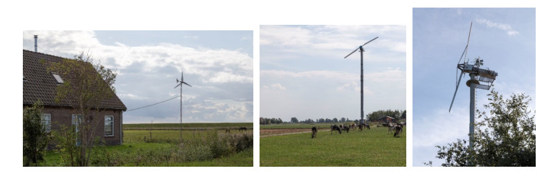
The paper deals with small wind turbines for grid-independent or small smart grid wind turbine systems. Not all small turbine manufacturers worldwide have access to the engineering capacity for designing an efficient turbine. The objective of this work is to provide an easy-to-handle integrated design and performance prediction method for wind turbines and to show exemplary applications.
The underlying model for the design and performance prediction method is based on an advanced version of the well-established blade-element-momentum theory, encoded in MATLAB™. Results are (i) the full geometry of the aerodynamically profiled and twisted blades which are designed to yield maximum power output at a given wind speed and (ii) the non-dimensional performance characteristics of the turbine in terms of power, torque and thrust coefficient as a function of tip speed ratio. The non-dimensional performance characteristics are the basis for the dimensional characteristics and the synthesis of the rotor to the electric generator with its load.
Two parametric studies illustrate typical outcomes of the design and performance prediction method: A variation of the design tip speed ratio and a variation of the number of blades. The predicted impact of those parameters on the non-dimensional performance characteristics agrees well with common knowledge and experience.
Eventually, an interplay of various designed turbine rotors and the given drive train/battery charger is simulated. Criterions for selection of the rotor are the annual energy output, the rotor speed at design wind speed as well as high winds, and the axial thrust exerted on the rotor by the wind. The complete rotor/drive train//battery charger assembly is tested successfully in the University of Siegen wind tunnel.
Citation: Stephen K. Musau, Kathrin Stahl, Kevin Volkmer, Nicholas Kaufmann, Thomas H. Carolus. A design and performance prediction method for small horizontal axis wind turbines and its application[J]. AIMS Energy, 2021, 9(5): 1043-1066. doi: 10.3934/energy.2021048
The paper deals with small wind turbines for grid-independent or small smart grid wind turbine systems. Not all small turbine manufacturers worldwide have access to the engineering capacity for designing an efficient turbine. The objective of this work is to provide an easy-to-handle integrated design and performance prediction method for wind turbines and to show exemplary applications.
The underlying model for the design and performance prediction method is based on an advanced version of the well-established blade-element-momentum theory, encoded in MATLAB™. Results are (i) the full geometry of the aerodynamically profiled and twisted blades which are designed to yield maximum power output at a given wind speed and (ii) the non-dimensional performance characteristics of the turbine in terms of power, torque and thrust coefficient as a function of tip speed ratio. The non-dimensional performance characteristics are the basis for the dimensional characteristics and the synthesis of the rotor to the electric generator with its load.
Two parametric studies illustrate typical outcomes of the design and performance prediction method: A variation of the design tip speed ratio and a variation of the number of blades. The predicted impact of those parameters on the non-dimensional performance characteristics agrees well with common knowledge and experience.
Eventually, an interplay of various designed turbine rotors and the given drive train/battery charger is simulated. Criterions for selection of the rotor are the annual energy output, the rotor speed at design wind speed as well as high winds, and the axial thrust exerted on the rotor by the wind. The complete rotor/drive train//battery charger assembly is tested successfully in the University of Siegen wind tunnel.

| [1] | European Commission, FP 7. Available from: https://cordis.europa.eu (assessed April 08, 2020). |
| [2] | RenewableUK, Small Wind Turbine Standard (15 January, 2014). Available from: https://mcscertified.com/wp-content/uploads/2019/08/RenewableUK-Small-Wind-Turbine-Standard-2014-01-05.pdf (assessed April 04, 2020). |
| [3] | Jütemann P, Kleinwind-Marktreport 2020. Available from: http://www.Klein-Windkraftanlagen.com ((assessed April 04, 2020). |
| [4] | ARGE Lichtenegg, Wien, Austria. Available from: http://www.energieforschungspark.at (assessed April 04, 2020). |
| [5] | Kaufmann N, "Small Horizontal Axis Free-Flow Turbines for Tidal Currents, " ISBN 978-3-8440-6705-7. Shaker-Verlag Düren, 2019. |
| [6] | Gasch R, Twele J (2013) Windkraftanlagen: Grundlagen, Entwurf, Planung und Betrieb. 8th ed. Stuttgart: Springer Vieweg. |
| [7] | Gerhard T, Sturm M, Carolus T (2013) Small Horizontal Axis Wind Turbine: Analytical Blade Design and Comparison with RANS-Prediction and Experimental Data. Proceedings of the ASME Turbo Expo 2013. |
| [8] | Betz A (1994) Windenergie und ihre Ausnutzung durch Windmühlen: 1926. Reprint Ö kobuch Freiburg, 1994. |
| [9] | Drela M (2013) XFOIL—Subsonic Airfoil Development System, 2013. |
| [10] | Drela M (2003) Implicit Implementation of the Full e.n Transition Criterion. In 21st AIAA Applied Aerodynamics Conference, Orlando, Florida, 2003. |
| [11] | Glauert H (1935) Airplane Propellers, in Aerodynamic Theory: A General Review of Progress Under a Grant of the Guggenheim Fund for the Promotion of Aeronautics. W. F. Durand, Ed., Berlin, Heidelberg: Springer Berlin Heidelberg, 169-360. |
| [12] | Sørensen JN (2016) General Momentum Theory for Horizontal Axis Wind Turbines. 1st ed. s.l.: Springer-Verlag, 2016. |
| [13] | Moriarty PJ, Hansen AC (2005) AeroDyn Theory Manual. Golden, CO: National Renewable Energy Laboratory, 2005. |
| [14] | Shen WZ, Mikkelsen R, Sørensen JN, et al. (2005) Tip loss corrections for wind turbine computations. Wind Energy 8: 457-475. |
| [15] | Buhl ML (2005) New Empirical Relationship between Thrust Coefficient and Induction Factor for the Turbulent Windmill State. Technical Report: NREL/TP-500-36834, National Renewable Energy Laboratory, Golden, CO, 2005. |
| [16] | Viterna LA, Corrigan RD (2008) Fixed pitch rotor performance of large horizontal axis wind turbines. In DOE/NASA Workshop on Large Horizontal Axis Wind Turbines, Cleveland, 1981. |
| [17] | MOL Hansen (2008) Aerodynamics of Wind Turbines. London: Earthscan, 2008. |
| [18] | DM Somers (2005), The S833, S834, and S835 Airfoils, National Renewable Energy Laboratory Report No. NREL/SR-500-36340, Golden, Colorado, USA 2005. |
| [19] | Chen Y, Mendoza ASE, Griffith DT, et al. (2021) Experimental and numerical study of high-order complex curvature mode shape and mode coupling on a three-bladed wind turbine assembly. Mech Syst Signal Process 160: 107873. |
| [20] | Chen Y, Joffre, Avitabile P (2018) Underwater dynamic response at limited points expanded to full —field strain response. J Vib Acoust, 2018. |
| [21] | Chen W, Jin M, Huang J, et al. (2021) A method to distinguish harmonic frequencies and remove the harmonic effect in operational modal analysis of rotating structures. Mech Syst Signal Process 161: 107928. |
| [22] | Ceyhan O (2008) Aerodynamic design and optimization axis wind turbines by using BEM theory and genetic Algorithm. |
| [23] | Clifton-Smith MJ, Wood DH (2007) Further Dual purpose evolutionary optimization of small wind turbine blades. J Phys Conf Ser. |
| [24] | Liu X, Chen Y, Ye Z (2007) Optimization model for rotor blades of horizontal axis wind turbines. Front Mech Eng 2: 483-488. |
| [25] | Lee MH, Shiah YC, Bai CJ (2016) Experiments and numerical simulations of the rotor blade performance for a small-scale horizontal axis wind turbine. J Wind Eng Ind Aerodyn 149: 17-29. |
| [26] | Lanazafame R, Messina M (2007) Fluid dynamics wind turbine design: Critical analysis, optimization and application of BEM theory. Renewable Energy 32: 2291-2305. |


Figures(14) / Tables(4)

Stephen K. Musau, Kathrin Stahl, Kevin Volkmer, Nicholas Kaufmann, Thomas H. Carolus. A design and performance prediction method for small horizontal axis wind turbines and its application[J]. AIMS Energy, 2021, 9(5): 1043-1066. doi: 10.3934/energy.2021048


 DownLoad: