Figure 1.
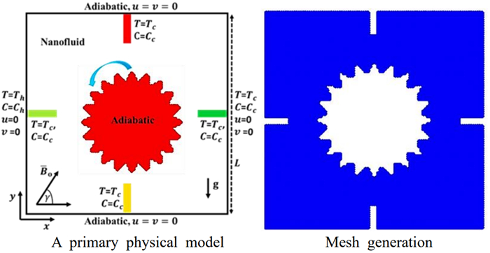
Primary model of rotated wavy cylinder and four fins in the cavity's center borders.


Due to high requirements of storage, operation and delivery conditions, it is more difficult for cold chain logistics to meet the demand with supply in the course of disruption. And, accurate demand forecasting promotes supply efficiency for cold chain logistics in a changeable environment. This paper aims to find the main influential factors of cold chain demand and presents a prediction to support the resilience operation of cold chain logistics. After analyzing the internal relevance between potential factors and regional agricultural cold chain logistics demand, the grey model GM (1, N) with fractional order accumulation is established to forecast future agricultural cold chain logistics demand in Beijing, Tianjin, and Hebei. The following outcomes have been obtained. (1) The proportion of tertiary industry, per capita disposable income indices for urban households and general price index for farm products are the first three factors influencing the cold chain logistics demand for agricultural products in both Beijing and Tianjin. The GDP, fixed asset investment in transportation and storage, and the proportion of tertiary industry are three major influential factors in Hebei. (2) Agricultural cold chain demand in Beijing and Hebei will grow sustainably in 2021–2025, while the trend in Tianjin remains stable. In conclusion, regional developmental differences should be considered when planning policies for the Beijing-Tianjin-Hebei cold chain logistics system.
Citation: Xiangyang Ren, Juan Tan, Qingmin Qiao, Lifeng Wu, Liyuan Ren, Lu Meng. Demand forecast and influential factors of cold chain logistics based on a grey model[J]. Mathematical Biosciences and Engineering, 2022, 19(8): 7669-7686. doi: 10.3934/mbe.2022360
| [1] | Giacomo Ascione, Enrica Pirozzi . On a stochastic neuronal model integrating correlated inputs. Mathematical Biosciences and Engineering, 2019, 16(5): 5206-5225. doi: 10.3934/mbe.2019260 |
| [2] | Virginia Giorno, Serena Spina . On the return process with refractoriness for a non-homogeneous Ornstein-Uhlenbeck neuronal model. Mathematical Biosciences and Engineering, 2014, 11(2): 285-302. doi: 10.3934/mbe.2014.11.285 |
| [3] | Meng Gao, Xiaohui Ai . A stochastic Gilpin-Ayala mutualism model driven by mean-reverting OU process with Lévy jumps. Mathematical Biosciences and Engineering, 2024, 21(3): 4117-4141. doi: 10.3934/mbe.2024182 |
| [4] | Buyu Wen, Bing Liu, Qianqian Cui . Analysis of a stochastic SIB cholera model with saturation recovery rate and Ornstein-Uhlenbeck process. Mathematical Biosciences and Engineering, 2023, 20(7): 11644-11655. doi: 10.3934/mbe.2023517 |
| [5] | Zhihao Ke, Chaoqun Xu . Structure analysis of the attracting sets for plankton models driven by bounded noises. Mathematical Biosciences and Engineering, 2023, 20(4): 6400-6421. doi: 10.3934/mbe.2023277 |
| [6] | Katrine O. Bangsgaard, Morten Andersen, James G. Heaf, Johnny T. Ottesen . Bayesian parameter estimation for phosphate dynamics during hemodialysis. Mathematical Biosciences and Engineering, 2023, 20(3): 4455-4492. doi: 10.3934/mbe.2023207 |
| [7] | Yongxin Gao, Shuyuan Yao . Persistence and extinction of a modified Leslie-Gower Holling-type Ⅱ predator-prey stochastic model in polluted environments with impulsive toxicant input. Mathematical Biosciences and Engineering, 2021, 18(4): 4894-4918. doi: 10.3934/mbe.2021249 |
| [8] | Xiaochen Sheng, Weili Xiong . Soft sensor design based on phase partition ensemble of LSSVR models for nonlinear batch processes. Mathematical Biosciences and Engineering, 2020, 17(2): 1901-1921. doi: 10.3934/mbe.2020100 |
| [9] | M. Nagy, M. H. Abu-Moussa, Adel Fahad Alrasheedi, A. Rabie . Expected Bayesian estimation for exponential model based on simple step stress with Type-I hybrid censored data. Mathematical Biosciences and Engineering, 2022, 19(10): 9773-9791. doi: 10.3934/mbe.2022455 |
| [10] | Aniello Buonocore, Luigia Caputo, Enrica Pirozzi, Maria Francesca Carfora . A simple algorithm to generate firing times for leaky integrate-and-fire neuronal model. Mathematical Biosciences and Engineering, 2014, 11(1): 1-10. doi: 10.3934/mbe.2014.11.1 |
Due to high requirements of storage, operation and delivery conditions, it is more difficult for cold chain logistics to meet the demand with supply in the course of disruption. And, accurate demand forecasting promotes supply efficiency for cold chain logistics in a changeable environment. This paper aims to find the main influential factors of cold chain demand and presents a prediction to support the resilience operation of cold chain logistics. After analyzing the internal relevance between potential factors and regional agricultural cold chain logistics demand, the grey model GM (1, N) with fractional order accumulation is established to forecast future agricultural cold chain logistics demand in Beijing, Tianjin, and Hebei. The following outcomes have been obtained. (1) The proportion of tertiary industry, per capita disposable income indices for urban households and general price index for farm products are the first three factors influencing the cold chain logistics demand for agricultural products in both Beijing and Tianjin. The GDP, fixed asset investment in transportation and storage, and the proportion of tertiary industry are three major influential factors in Hebei. (2) Agricultural cold chain demand in Beijing and Hebei will grow sustainably in 2021–2025, while the trend in Tianjin remains stable. In conclusion, regional developmental differences should be considered when planning policies for the Beijing-Tianjin-Hebei cold chain logistics system.
The smoothed particle hydrodynamics (SPH) method is a Lagrangian representation that is based on a particle interpolation to calculate smooth field variables [1,2]. Because of its Lagrangian features, the SPH method has fine advantages. The SPH method is used to simulate several industrial applications by simulating highly dynamic and violent flows such as tank sloshing, oil flow in gearboxes, nozzles, and jet impingement. In addition, the SPH method works well with the free surface flows, surface tension in free surface flows, and breaking waves without a special treatment required in this area. Additionally, the simulations of multiphase flows are easily handled by the SPH method. In conventional grid-based approaches, both the Volume-of-Fluid (VOF) method and the Level set method are adept at accurately capturing multiphase interfaces. An additional strength of the SPH method is its ability to handle complex/moving geometries. He et al. [3] introduced a new, weakly-compressible, SPH model tailored for multi-phase flows with notable differences in the density, while also allowing for large Courant-Friedrichs-Lewy numbers. Their method involves adjusting the continuity equation to exclude contributions from particles of different phases, solely focusing on neighboring particles of the same phase. Subsequently, they utilize a Shepard interpolation to reset the pressure and density of the particles from other phases. Bao et al. [4] presented an upgraded method within the SPH aimed at simulating turbulent flows near walls with medium to high Reynolds numbers. Their approach combined the κ−ε turbulence model and a wall function to enhance the accuracy. To tackle numerical errors and challenges related to the boundary conditions, they split the second-order partial derivative term of the composite function containing the turbulent viscosity coefficient into two components. Ensuring uniform particles, smooth pressure fields, and efficient computation, they employed particle shifting techniques, the δ -SPH method, and graphics processing unit (GPU) parallel processing in their simulations. Huang et al. [5] devised an innovative approach that merged SPH with the Finite Difference Method (SPH-FDM) within an Eulerian framework to analyze the unsteady flow around a pitching airfoil. They introduced an improved Iterative Shifting Particle Technology (IPST) to accurately track the motion of pitching airfoils. The numerical results from the SPH-FDM approach within a Eulerian framework closely aligned with those from either the finite volume method (FVM) or the existing literature, affirming the effectiveness of their proposed method. Further applications of the SPH method and its incompressible scheme, entitled the ISPH method, can be found in the references [6,7,8,9,10,11,12,13,14,15,16,17]. In recent years, the ISPH-FVM coupling method refers to the integration of the ISPH method with the FVM. This hybrid approach combines the strengths of both techniques to accurately model the fluid flow phenomena, particularly in scenarios involving either complex geometries or multiphase flows. Xu et al. [18] introduced the ISPH-FVM coupling method to simulate a two-phase incompressible flow, and combined the advantages of ISPH in interface tracking and FVM in flow field calculations with enhancements in surface tension calculations inspired by VOF and Level Set methods, demonstrating an improved accuracy and stability in complex two-phase flow scenarios. Xu et al. [19] developed a 3D ISPH-FVM coupling technique to model a bubble ascent in a viscous stagnant liquid, and employed an exchange of information at overlapping regions between the ISPH and FVM schemes, with an evaluation of surface tension effects using the 3D continuum surface force model (CSF). They validated the accuracy of the interface capture through benchmark tests and compared simulations of a single bubble ascent against experimental and literature-based data; moreover, they explored the method's capabilities in various parameter settings and in studying the dynamics of a two-bubble coalescence, demonstrating the reliability and versatility of the approach in simulating the bubble ascent phenomena. Xu et al. [20] proposed an advanced mapping interpolation ISPH-FVM coupling technique tailored to simulate complex two-phase flows characterized by intricate interfaces. The nanofluids were a suspension of nanomaterials in the base fluids. The nanofluids were applied to enhance the thermal features of cooling devices and equipment in electronic cooling systems [21,22] and heat exchangers [23,24]. In 1995, Choi and Eastman [25] achieved an enhanced heat transfer by adding nanoparticles inside a base fluid. The double diffusion of nanofluids (Al2O3-H2O) in an enclosure under the magnetic field impacts was studied by the lattice Boltzmann method [26]. There are several uses of coupling magnetic field impacts on nanofluids in thermal engineering experiments [27,28,29,30,31,32]. The variable magnetic field on ferrofluid flow in a cavity was studied numerically by the ISPH method [33]. Aly [16] adopted the ISPH method to examine the effects of Soret-Dufour numbers and magnetic fields on the double diffusion from grooves within a nanofluid-filled cavity. To enhance the heat transfer in cavities, the wavy or extended surface or fins were applied. The fins were used in several mechanical engineering applications. Saeid [34] studied the existence of different fin shapes on a heating cavity. The numerical attempt based on the finite volume method was introduced for natural convection and thermal radiation in a cavity containing N thin fins [35]. Hussain et al. [36] examined the effects of fins and inclined magnetic field on mixed convection of a nanofluid inside single/double lid-driven cavities. The recent numerical attempts based on the ISPH method for double diffusion of a nanofluid in a finned cavity, which were introduced by Aly et al. [37,38]. This work examines the impacts of Cattaneo-Christov heat flux and magnetic impacts on the double diffusion of a nanofluid-filled cavity. The cavity contains a rotated wavy circular cylinder and four fins fixed on its borders. The ISPH method is utilized to handle the interactions between the rotational speed of an inner wavy cylinder with a nanofluid flow. The established ANN model can accurately predict the values of −Nu and −Sh, as demonstrated in this study, in which there is a high agreement between the prediction values generated by the ANN model and the target values.
The initial physical model and its particle generation are represented in Figure 1. The physical model contains a square cavity filled with a nanofluid and containing four fins and a wavy circular cylinder. The embedded wavy circular cylinder rotates around its center by a rotational velocity V=ω(r−r0) with adiabatic thermal/solutal conditions. The four fins are fixed at the center of the cavity borders with a low temperature/concentration Tc&Cc. The source is located on the left wall of a cavity with Th&Ch, the plane walls are adiabatic, and the right wall is maintained at Tc&Cc. It is assumed that the nanofluid flow is laminar, unsteady, and incompressible. Figure 2 depicts the architecture and fundamental configuration structure of the created multilayer perceptron (MLP) network. A model with 14 neurons in the hidden layer of the MLP network model was identified so that the number of neurons were included in the hidden layer [39,40]. To build ANN models, the data-collecting process must be idealistically structured. Three methods were used to arrange the 1, 020, 888 data points that were used to construct the ANN model. In the created MLP network model, the −Nu and −Sh values were estimated in the output layer, while the τ and Sr values were defined as input parameters in the input layer. A total of 70% of the data was set aside for model training, 15% for validation, and 15% for testing. The recommended training algorithm in the network model was the Levenberg-Marquardt (LM) algorithm. The LM algorithm effectively minimizes nonlinear least squares problems by iteratively adjusting parameters based on an objective function, utilizing the gradient descent and Gauss-Newton methods, while dynamically controlling the step size to prevent overshooting; this achieves convergence to the optimal parameter values, making it widely used in various fields for an efficient optimization. Below are the transfer functions that are employed in the MLP network's hidden and output layers:
| f(x)=21+e(−2x)−1 | (1) |
| purelin(x)=x. | (2) |
The mathematical equations utilized to compute the mean squared error (MSE), coefficient of determination (R), and margin of deviation (MoD) values, which were selected as the performance criteria, are outlined below [41]:
| MSE=1N∑Ni=1(Xtarg(i)−Xpred(i))2 | (3) |
| R=√1−∑Ni=1(Xtarg(i)−Xpred(i))2∑Ni=1(Xtarg(i))2 | (4) |
| MoD(%)=[Xtarg−XpredXtarg]x100. | (5) |

The regulating equations in the Lagrangian description [38,42,43] are as follows:
| ∂u∂x+∂v∂y=0, | (6) |
| dudt=−1ρnf∂p∂x+μnfρnf(∂2u∂x2+∂2u∂y2)−σnfB20ρnf(usin2γ−vsinγcosγ), | (7) |
| dvdt=−1ρnf∂p∂y+μnfρnf(∂2v∂x2+∂2v∂y2)+(ρβT)nfρnfg(T−Tc)+(ρβC)nfρnfg(C−Cc)−σnfB20ρnf(vcos2γ−usinγcosγ), | (8) |
| dTdt=∇·(αnf∇T)+1(ρCP)nf∇·(D1∇C)−δ1(u∂T∂x∂u∂x+v∂T∂y∂v∂y+u2∂2T∂x2+v2∂2T∂y2+2uv∂2T∂x∂y+u∂T∂y∂v∂x+v∂T∂x∂u∂y), | (9) |
| dCdt=∇·(Dm∇C)+∇·(D2∇T). | (10) |
The dimensionless quantities [38,42,43] are as follows:
| X=xL,Y=yL,τ=tαfL2,U=uLαf,V=vLαf,αf=kf(ρCP)f |
| P=pL2ρnfα2f,θ=T−TcTh−Tc,Φ=C−CcCh−Cc. | (11) |
After substituting Eq (6) into the dimension form of governing Eqs (1)-(5), then the dimensionless equations [38,42,43] are as follows:
| ∂U∂X+∂V∂Y=0, | (12) |
| dUdτ=−∂P∂X+μnfρnfαf(∂2U∂X2+∂2U∂Y2)−σnfρfσfρnfHa2Pr(Usin2γ−Vsinγcosγ), | (13) |
| dVdτ=−∂P∂Y+μnfρnfαf(∂2V∂X2+∂2V∂Y2)+(ρβ)nfρnfβfRaPr(θ+NΦ)−σnfρfσfρnfHa2Pr(Vcos2γ−Usinγcosγ), | (14) |
| dθdτ=1(ρCP)nfDu(∂2Φ∂X2+∂2Φ∂Y2)+αnfαf(∂2θ∂X2+∂2θ∂Y2)−δC(U∂θ∂X∂U∂X+V∂θ∂Y∂V∂Y+U2∂2θ∂X2+V2∂2θ∂Y2+2UV∂2θ∂X∂Y+U∂θ∂Y∂V∂X+V∂θ∂X∂U∂Y), | (15) |
| dΦdτ=Sr(∂2θ∂X2+∂2θ∂Y2)+1Le(∂2Φ∂X2+∂2Φ∂Y2). | (16) |
The Soret number is Sr=D2αf((Th−Tc)(Ch−Cc)), δC=νfδ1L2 is the Cattaneo Christov heat flux parameter, and Du=D1αf((Ch−Cc)(Th−Tc)) is Dufour number. The Hartmann number is Ha=√σfμfB0L, the buoyancy ratio is N=βC(Ch−Cc)βT(Th−Tc), Rayleigh's number is Ra=gβT(Th−Tc)L3νfαf, the Prandtl number is Pr=νfαf, and Lewis's number is Le=αfDm.
Left wall, θ=Φ=1,U=0=V, (17)
Right wall, θ=Φ=0,U=0=V,
Plane walls, ∂Φ∂Y=∂θ∂Y=0,U=0=V,
Four fins, θ=Φ=0,U=0=V,
Wavy circular cylinder ∂Φ∂Y=∂θ∂Y=0,U=Urot,V=Vrot,
The mean Nusselt/Sherwood numbers are as follows:
| −Nu=−∫10knfkf(∂θ∂X)dY, | (18) |
| −Sh=−∫10(∂Φ∂X)dY. | (19) |
The nanofluid properties are as follows ([44,45,46]):
| ρnf=ρf−ϕρf+ϕρnp | (20) |
| (ρCp)nf=(ρCp)f−ϕ(ρCp)f+ϕ(ρCp)np | (21) |
| (ρβ)nf=ϕ(ρβ)np−ϕ(ρβ)f+(ρβ)f | (22) |
| σnf=σf(1+3ϕ(σnp/σf−1)(σnp/σf+2)−(σnp/σf−1)ϕ) | (23) |
| αnf=knf(ρCp)nf | (24) |
| knf=(knp+2kf)+ϕ((knp+2kf)kf−2ϕ(kf−knp)kf)(kf−knp)−1 | (25) |
| μnf=(1−ϕ)−2.5μf. | (26) |
The solving steps in the ISPH method [42,43,47,48] are as follows:
First:
| U∗=μnfΔτρnfαf(∂2U∂X2+∂2U∂Y2)n−ΔτσnfρfσfρnfHa2Pr(Unsin2γ−Vnsinγcosγ)+Un | (27) |
| V∗=μnfΔτρnfαf(∂2V∂X2+∂2V∂Y2)n−ΔτσnfρfσfρnfHa2Pr(Vncos2γ−Unsinγcosγ)+Δτ(ρβ)nfρnfβfRaPr(θn+NΦn)+Vn. | (28) |
Second:
| ∇2Pn+1=1Δτ(∂U∗∂X+∂V∗∂Y). | (29) |
Third:
| Un+1=U∗−Δτ(∂P∂X)n+1, | (30) |
| Vn+1=V∗−Δτ(∂P∂Y)n+1. | (31) |
Fourth:
| θn+1=θn+αnfΔταf(∂2θ∂X2+∂2θ∂Y2)n+Δτ(ρCP)nfDu(∂2Φ∂X2+∂2Φ∂Y2)n−ΔτδC(U∂θ∂X∂U∂X+V∂θ∂Y∂V∂Y+U2∂2θ∂X2+V2∂2θ∂Y2+2UV∂2θ∂X∂Y+U∂θ∂Y∂V∂X+V∂θ∂X∂U∂Y)n, | (32) |
| Φn+1=Φn+ΔτLe(∂2Φ∂X2+∂2Φ∂Y2)n+ΔτSr(∂2θ∂X2+∂2θ∂Y2)n. | (33) |
Fifth:
| rn+1=ΔτUn+1+rn. | (34) |
The shifting technique [49,50] is as follows:
| ϕi'=ϕi+(∇ϕ)i·δrii'+O(δr2ii'). | (35) |
The ISPH method's flowchart encompasses initiating the computational domain and boundary conditions, advancing through the time steps to estimate particle densities, solving the pressure fields, computing the heat and mass transfer, updating the particle velocities and positions, and ultimately analyzing results, all to accurately simulate the fluid dynamics. The flowchart of the ISPH method is shown in Figure 3.

This section introduces several numerical tests of the ISPH approach, beginning with an examination of the natural convection around a circular cylinder within a square cavity. Figure 4 illustrates a comparison of isotherms during the natural convection (NC) at different Rayleigh numbers (Ra) between the ISPH approach and the numerical findings by Kim et al. [51]. The ISPH approach yielded results consistent with those obtained by Kim et al. [51].

Second, the ISPH method's validation for the natural convection in a cavity with a heated rectangle source is presented. Figure 5 compares the ISPH method with numerical simulations (Fluent software) and experimental data from Paroncini and Corvaro [51] for isotherms at various Rayleigh numbers and hot source heights. The ISPH method shows good agreement with both experimental and numerical results across different scenarios. Additionally, Figure 6 illustrates comparisons between the experimental, numerical, and ISPH method results for streamlines at different Rayleigh numbers and hot source lengths, confirming the accuracy of the ISPH method simulations without redundancy.


The performed numerical simulations are discussed in this section. The range of pertinent parameters is the Cattaneo Christov heat flux parameter (0≤δc≤0.001), the Dufour number (0≤Du≤2), the nanoparticle parameter (0≤ϕ≤0.1), the Soret number (0≤Sr≤2), the Hartmann number (0≤Ha≤80), the Rayleigh number (103≤Ra≤105), Fin's length (0.05≤LFin≤0.2), and the radius of a wavy circular cylinder (0.05≤RCyld≤0.3). Figure 7 shows the effects of δc on the temperature θ, concentration Φ, and velocity field V. Increasing δc slightly enhances the temperature, concentration, and velocity field within an annulus. Figure 8 shows the effects of Du on θ, Φ, and V. Physically, the Dufour number indicates the influence of concentration gradients on thermal energy flux. An increase in Du has a minor influence on θ and Φ. Increasing Du growths the velocity field. These results are relevant to the presence of a diabatic wavy cylinder inside a square cavity, which shrinks the contributions of Du. Figure 9 represents the effects of Ha on θ, Φ, and V. The Hartmann number (Ha) is a proportion of an electromagnetic force to a viscous force. Physically, the Lorentz forces represent the magnetic field that shrinks the flow velocity. Consequently, an increment in Ha shrinks the distributions of θ and Φ. The maximum of the velocity field declines by 87.09% as Ha powers from 0 to 80. The study of the inner geometric parameters including the length of inner fins LFin and the radius of a wavy circular cylinder RCyld on the features of temperature, concentration, and velocity field is represented in Figures 10 and 11. In Figure 10, an expanded of LFin supports the cooling area, which reduces the strength of θ and Φ within a cavity. As the inner fins represent blockages for the nanofluid flow in a square cavity, the maximum of the velocity field reduces by 48.65% as the LFin boosts from 0.05 to 0.2. In Figure 11, regardless of the adiabatic condition of an inner wavy cylinder, an increment in RCyld reduces the distributions of temperature and concentration across the cavity. Furthermore, due to the low rotating speed of the inner wavy cylinder, an expanded wavy cylinder reduces the velocity field. It is seen that the maximum of the velocity field shrinks by 55.42% according to an increase in RCyld from 0.05 to 0.3. Figure 12 represents the effects of ϕ on θ, Φ, and V. Here, due to the presence of an inner wavy cylinder, the contribution of ϕ is minor in enhancing the cooling area and reducing the strength of the concentration inside a cavity, whilst the physical contribution of ϕ in increasing the viscosity of a nanofluid appears well by majoring the velocity field. The velocity's maximum reduces by 36.52% according to an increasing concentration of nanoparticles from 0 to 10%. Figure 13 establishes the effects of Ra on θ, Φ, and V. As Ra represents the ratio of buoyancy to thermal diffusivity and it is considering a main factor in controlling the natural convection. Accordingly, there are beneficial enhancements in the strength of the temperature and concentration in a cavity according to an increase in Ra. Furthermore, the Rayleigh number effectively works to accelerate the velocity field in a cavity. Figure 14 indicates the effects of Sr on θ, Φ, and V. Physically, the Soret influence expresses diffusive movement that is created from a temperature gradient. Increasing Sr enhances the strength of the temperature; this increment strongly enhances the strength of the concentration. Increasing Sr from 0 to 2 supports the velocity's maximum by 134.3%. Figure 15 indicates the average −Nu and −Sh under the variations of Sr, RCyld, Ha, and δC. The average −Nu is enhanced according to an increment in Sr, whilst it decreases alongside an increase in RCyld and Ha. The average −Sh decreases alongside an increase of Sr, RCyld, and Ha. It is found that the variations of δC slightly changes the values of −Nu and −Sh.


Figure 16 displays the performance chart that was made to examine the produced ANN model's training phase. The graph illustrates how the MSE values, which were large at the start of the training phase, got smaller as each epoch progressed. By achieving the optimal validation value for each of the three data sets, the MLP model's training phase was finished. The error histogram derived from the training phase's data is displayed in Figure 17. Upon scrutinizing the error histogram, one observes that the error values are predominantly centered around the zero-error line. Additionally, relatively low numerical values for the errors were achieved. In Figure 18, the regression curve for the MLP model is displayed, indicating that R = 1 is consistently employed for training, validation, and testing. According to the results of the performance, regression, and error histograms, the built ANN model's training phase was successfully finished. Following the training phase's validation, the ANN model's prediction performance was examined. First, the goal values and the −Nu and −Sh values derived by the ANN model were compared in this context. The goal values for every data point are displayed in Figure 19, along with the −Nu and −Sh values that the ANN model produced. Upon a closer inspection of the graphs, it becomes evident that the −Nu and −Sh values derived by the ANN model perfectly align with the desired values.


The current work numerically examined the effects of a Cattaneo-Christov heat flux on the thermosolutal convection of a nanofluid-filled square cavity. The square cavity had four fins located on the cavity's boarders and a wavy circular cylinder, which was located in the cavity's center, and rotated in a circular form. This study checked the impacts of the Cattaneo Christov heat flux parameter, the Dufour number, a nanoparticle parameter, the Soret number, the Hartmann number, the Rayleigh number, Fin's length, and the radius of a wavy circular cylinder on the temperature, concentration, and velocity field. The results are highlighted within the following points:
• The parameters of the embedded blockages, including the fins length and radius of a wavy circular cylinder, worked well to improve the cooling area and reduce the strength of concentration as well as the velocity field.
• Adding an extra concentration of nanoparticles up to 10% enhanced the cooling area and reduced the maximum velocity field by 36.52%.
• The Rayleigh number beneficially contributed to power the double diffusion within an annulus and was effective in accelerating the nanofluid velocity.
• The Soret number effectively contributed to change the distributions of the temperature, the concentration, and the velocity field within an annulus as compared to the Dufour number.
• The excellent accord between the prediction values produced by the ANN model and the goal values indicated that the developed ANN model could forecast the −Nu and −Sh values with a remarkable precision.
Munirah Alotaibi: Conceptualization, Funding acquisition, Methodology, Writing – original draft; Abdelraheem M. Aly: Formal Analysis, Investigation, Validation, Visualization, Writing – review & editing. All authors have read and approved the final version of the manuscript for publication.
The authors declare they have not used Artificial Intelligence (AI) tools in the creation of this article.
The authors extend their appreciation to the Deanship of Scientific Research at King Khalid University, Abha, Saudi Arabia, for funding this work through the Research Group Project under Grant Number (RGP. 2/38/45). This research was funded by the Princess Nourah bint Abdulrahman University Researchers Supporting Project number (PNURSP2024R522), Princess Nourah bint Abdulrahman University, Riyadh, Saudi Arabia.
The authors declare that they have NO affiliations with or involvement in any organization or entity with any financial interest.
| [1] |
D. Samson, Operations/supply chain management in a new world context, Oper. Manage. Res. Adv. Pract. Theory, 13 (2020), 1-3. https://doi.org/10.1007/s12063-020-00157-w doi: 10.1007/s12063-020-00157-w

|
| [2] |
O. Theophilus, M. A. Dulebenets, J. Pasha, Y. Lau, A. M. Fathollahi-Fard, A. Mazaheri, Truck scheduling optimization at a cold-chain cross-docking terminal with product perishability considerations, Comput. Ind. Eng., 1 (2021), 107240. https://doi.org/10.1016/j.cie.2021.107240 doi: 10.1016/j.cie.2021.107240
|
| [3] |
J. Wang, R. R. Muddada, H. Wang, J. Ding, Y. Lin, C. Liu, et al., Toward a resilient holistic supply chain network system: Concept, review and future direction, IEEE Syst. J., 10 (2016), 410-421. https://doi.org/10.1109/JSYST.2014.2363161 doi: 10.1109/JSYST.2014.2363161
|
| [4] |
J. Blackburn, G. Scudder, Supply chain strategies for perishable products: The case of fresh produce, Prod. Oper. Manage., 18 (2009), 129-137. https://doi.org/10.1111/j.1937-5956.2009.01016.x doi: 10.1111/j.1937-5956.2009.01016.x
|
| [5] |
R. Haass, P. Dittmer, M. Veigt, M. Lütjen, Reducing food losses and carbon emission by using autonomous control-A simulation study of the intelligent container, Int. J. Prod. Econ., 164 (2015), 400-408. https://doi.org/10.1016/j.ijpe.2014.12.013 doi: 10.1016/j.ijpe.2014.12.013
|
| [6] |
J. Fu, D. Yang, The current situation, dilemma and policy suggestions of China's cold chain logistics development, China Econ. Trade Herald, 9 (2021), 20-23. https://doi.org/10.3969/j.issn.1007-9777.2021.13.006 doi: 10.3969/j.issn.1007-9777.2021.13.006
|
| [7] |
C. Mena, L. A. Terry, L. Ellram, Causes of waste across multi-tier supply networks: Cases in the UK food sector, Int. J. Prod. Econ., 152 (2014), 144-158. https://doi.org/10.1016/j.ijpe.2014.03.012 doi: 10.1016/j.ijpe.2014.03.012
|
| [8] |
F. Zheng, Y. Pang, Y. Xu, M. Liu, Heuristic algorithms for truck scheduling of cross-docking operations in cold-chain logistics, Int. J. Prod. Res., 59 (2021), 6579-6600. https://doi.org/10.1080/00207543.2020.1821118 doi: 10.1080/00207543.2020.1821118
|
| [9] |
F. Pan, T. Fan, X. Qi, J. Chen, C. Zhang, Truck scheduling for cross-docking of fresh produce with repeated loading, Math. Problems Eng., 2021 (2021). https://doi.org/10.1155/2021/5592122 doi: 10.1155/2021/5592122
|
| [10] |
M. A. Dulebenets, E. E. Ozguven, R. Moses, M. B. Ulak, Intermodal freight network design for transport of perishable products, Open J. Optim., 5 (2016), 120-139. https://doi.org/10.4236/ojop.2016.54013 doi: 10.4236/ojop.2016.54013
|
| [11] |
C. Qi, L. Hu, Optimization of vehicle routing problem for emergency cold chain logistics based on minimum loss, Phys. Commun., 40 (2020), 101085. https://doi.org/10.1016/j.phycom.2020.101085 doi: 10.1016/j.phycom.2020.101085
|
| [12] |
M. A. Dulebenets, E. E. Ozguven, Vessel scheduling in liner shipping: Modeling transport of perishable assets, Int. J. Prod. Econ., 184 (2017), 141-156. https://doi.org/10.1016/j.ijpe.2016.11.011 doi: 10.1016/j.ijpe.2016.11.011
|
| [13] |
M. Wang, X. Li, Demand forecasting of agricultural cold chain logistics based on metabolic GM (1, 1) model. IOP Conf. Series Earth Environ. Sci., 831 (2021). https://doi.org/10.1016/10.1088/1755-1315/831/1/012018 doi: 10.1016/10.1088/1755-1315/831/1/012018
|
| [14] |
T. Liu, S. Li, S. Wei, Forecast and opportunity analysis of cold chain logistics demand of fresh agricultural products under the integration of Beijing, Tianjin and Hebei. Open J. Social Sci., 5 (2017), 63-73. https://doi.org/10.4236/jss.2017.510006 doi: 10.4236/jss.2017.510006
|
| [15] |
B. He, L. Yin, Z. Ernesto, Prediction modelling of cold chain logistics demand based on data mining algorithm, Math. Probl. Eng., 2021 (2021). https://doi.org/10.1155/2021/3421478 doi: 10.1155/2021/3421478
|
| [16] |
S. Wang, C. Wei, Demand prediction of cold chain logistics under B2C E-Commerce model, J. Adv. Comput. Intell. Intell. Inf., 22 (2018), 1082-1087. https://doi.org/10.20965/jaciii.2018.p1082 doi: 10.20965/jaciii.2018.p1082
|
| [17] | R. Xu, H. Lan, Demand forecasting model of aquatic cold chain logistics based on GWO-SVM, in Conference Proceedings of the 8th International Symposium on Project Management, (2020), 1088-1093. https://doi.org/10.26914/c.cnkihy.2020.029466 |
| [18] |
M Wang, X. Li, Demand forecasting of agricultural cold chain logistics based on metabolic GM (1, 1) model, IOP Conf. Ser. Earth Environ. Sci., 831 (2021). https://doi.org/10.1088/1755-1315/831/1/012018 doi: 10.1088/1755-1315/831/1/012018
|
| [19] | J. Lv, Y. Chen, Dalian aquatic products cold chain logistics demand forecast and analysis of influencing factors, Math. Pract. Theory, (2020), 72-80 |
| [20] |
B. Ya, Study of food cold chain logistics demand forecast based on multiple regression and AW-BP forecasting method on system order parameters, J. Comput. Theor. Nanosci., 13 (2016), 4019-4024. https://doi.org/10.1166/jctn.2016.4930 doi: 10.1166/jctn.2016.4930
|
| [21] |
C. Bu, L. Chen, Demand forecast of cold chain logistics of fresh agricultural products in Jiangsu province based on GA-BP model, World Sci. Res. J., 7 (2021), 210-217. https://doi.org/10.6911/WSRJ.202108_7(8).0034 doi: 10.6911/WSRJ.202108_7(8).0034
|
| [22] | J. L. Deng, An introduction to grey mathematics-grey hazy set, Huazhong University of Science and Technology Press, 1992 |
| [23] |
L. Wu, S. Liu, L. Yao, S. Yan, D. Liu, Grey system model with the fractional order accumulation, Commun. Nonlinear Sci. Numer. Simul., 18 (2013), 1775-1785. https://doi.org/10.1016/j.cnsns.2012.11.017 doi: 10.1016/j.cnsns.2012.11.017
|
| [24] |
L. Wu, S. Liu, Z. Fang, H. Xu, Properties of the GM (1, 1) with fractional order accumulation, Appl. Math. Comput., 252 (2015), 287-293. https://doi.org/10.1016/j.amc.2014.12.014 doi: 10.1016/j.amc.2014.12.014
|
| [25] |
Z. X. Wang, P. Hao, An improved grey multivariable model for predicting industrial energy consumption in China, Appl. Math. Model., 40 (2016), 5745-5758. https://doi.org/10.1016/j.apm.2016.01.012 doi: 10.1016/j.apm.2016.01.012
|
| [26] |
H. Chen, Y. Tong, L. Wu, Forecast of energy consumption based on FGM (1, 1) model, Math. Probl. Eng., 2021 (2021). https://doi.org/10.1155/2021/6617200 doi: 10.1155/2021/6617200
|
| [27] |
Y. Xu, T. S. Lim, K. Wang, Prediction of farmers' income in Hebei province based on the fractional grey model (1, 1), J. Math., 2021 (2021). https://doi.org/10.1155/2021/4869135 doi: 10.1155/2021/4869135
|
| [28] | S. Mao, X. Xiao, M. Gao, X. Wang, Nonlinear fractional order grey model of urban traffic flow short-term prediction, J. Grey Syst., 30 (2018), 1-17 |
| [29] | X. Qin, H. Tian, Comprehensive evaluation of cold chain logistics level of agricultural products in China based on grey cluster analysis, Preserv. Process., 19 (2019), 170-177 |
| [30] | S. Liu, Y. Yang, L. Wu, The grey system theory and application, Science Press, 2014. |
| [31] |
J. Wang, N. Li, Influencing factors and future trends of natural gas demand in the eastern, central and western areas of China based on the grey model, Nat. Gas Ind. B, 7 (2020). https://doi.org/10.1016/j.ngib.2020.09.005 doi: 10.1016/j.ngib.2020.09.005
|
| [32] |
L. Wu, S. Liu, Z. Fang, H. Xu, Properties of the GM (1, 1) with fractional order accumulation, Appl. Math. Comput., 252 (2015), 287-293. https://doi.org/10.1016/j.amc.2014.12.014 doi: 10.1016/j.amc.2014.12.014
|
| [33] |
S. Lan, C. Yang, G. Q. Huang, Data analysis for metropolitan economic and logistics development, Adv. Eng. Inf., 32 (2017), 66-76. https://doi.org/10.1016/j.aei.2017.01.003 doi: 10.1016/j.aei.2017.01.003
|
| [34] |
W. Zhang, X. Zhang, M. Zhang, W. Li, How to coordinate economic, logistics and ecological environment? Evidences from 30 provinces and cities in China, Sustainability, 12 (2020), 1058. https://doi.org/10.3390/su12031058 doi: 10.3390/su12031058
|
| [35] |
R. Xie, H. Huang, Y. Zhang, P. Yu, Coupling relationship between cold chain logistics and economic development: A investigation from China, PloS one, 17 (2022), e0264561-e0264561. https://doi.org/10.1371/JOURNAL.PONE.0264561 doi: 10.1371/JOURNAL.PONE.0264561
|
| [36] |
J. Li, L. Sun, Demand forecast of the cold chain logistics based on the multiple linear regression analysis, J. Anhui Agric. Sci., 39 (2011), 6519-6520. https://doi.org/10.13989/j.cnki.0517-6611.2011.11.142 doi: 10.13989/j.cnki.0517-6611.2011.11.142
|
| [37] |
T. Rossi, R. Pozzi, G. Pirovano, R. Cigolini, M. Pero, A new logistics model for increasing economic sustainability of perishable food supply chains through intermodal transportation, Int. J. Logistics Res. Appl., 24 (2020), 1-18. https://doi.org/10.1080/13675567.2020.1758047 doi: 10.1080/13675567.2020.1758047
|
| [38] |
M. Li, J. Wang, Prediction of demand for cold chain logistics of aquatic products based on RBF nueral network, Chin. J. Agric. Resour. Reg. Plann., 41 (2020), 10. https://doi.org/10.7621/cjarrp.1005-9121.20200612 doi: 10.7621/cjarrp.1005-9121.20200612
|
| [39] |
X. Wang, K. Zhao, Forecast of logistics demand of agricultural products based on neural network, J. Agrotechnical Econ., 2 (2010), 62-68. https://doi.org/10.13246/j.cnki.jae.2010.02.006 doi: 10.13246/j.cnki.jae.2010.02.006
|
| [40] |
L. Wu, S. Liu, L. Yao, S. Yan, The effect of sample size on the grey system model, Appl. Math. Model., 37 (2013), 6577-6583. https://doi.org/10.1016/j.apm.2013.01.018 doi: 10.1016/j.apm.2013.01.018
|
| [41] |
C. Magazzino, M. Mele, On the relationship between transportation infrastructure and economic development in China, Res. Transp. Econ., 88 (2020), 100947. https://doi.org/10.1016/j.retrec.2020.100947 doi: 10.1016/j.retrec.2020.100947
|
| [42] |
J. Li, Research on development strategy of cold chain logistics based on food safety, Front. Econ. Manage., 2 (2021), 214-225. https://doi.org/10.6981/FEM.202103_2(3).0028 doi: 10.6981/FEM.202103_2(3).0028
|
| [43] |
B. Mary, O. Akinola, W. Zhang, A systems dynamics approach to the management of material procurement for engineering, procurement and construction industry, Int. J. Prod. Econ., 244 (2022). https://doi.org/10.1016/J.IJPE.2021.108390 doi: 10.1016/J.IJPE.2021.108390
|
| [44] |
J. W. Wang, W. H. lp, R. R. Muddada, J. L. Huang, W. J. Zhang, On Petri net implementation of proactive resilient holistic supply chain networks, Int. J. Adv. Manuf. Technol., 69 (2013), 427-437. https://doi.org/10.1007/s00170-013-5022-x doi: 10.1007/s00170-013-5022-x
|


Figures(2) / Tables(11)

Xiangyang Ren, Juan Tan, Qingmin Qiao, Lifeng Wu, Liyuan Ren, Lu Meng. Demand forecast and influential factors of cold chain logistics based on a grey model[J]. Mathematical Biosciences and Engineering, 2022, 19(8): 7669-7686. doi: 10.3934/mbe.2022360

 DownLoad:
