Research article Special Issues

On a stochastic neuronal model integrating correlated inputs

  • A modified LIF-type stochastic model is considered with a non-delta correlated stochastic process in place of the traditional white noise. Two different mechanisms of reset are specified with the aim to model endogenous and exogenous correlated input stimuli. Ornstein-Uhlenbeck processes are used to model the two different cases. An equivalence between different ways to include currents in the model is also shown. The theory of integrated stochastic processes is evoked and the main features of involved processes are obtained, such as mean and covariance functions. Finally, a simulation algorithm of the proposed model is described; simulations are performed to provide estimations of firing densities and related comparisons are given.

    Citation: Giacomo Ascione, Enrica Pirozzi. On a stochastic neuronal model integrating correlated inputs[J]. Mathematical Biosciences and Engineering, 2019, 16(5): 5206-5225. doi: 10.3934/mbe.2019260

    Related Papers:

    [1] Virginia Giorno, Serena Spina . On the return process with refractoriness for a non-homogeneous Ornstein-Uhlenbeck neuronal model. Mathematical Biosciences and Engineering, 2014, 11(2): 285-302. doi: 10.3934/mbe.2014.11.285
    [2] Aniello Buonocore, Luigia Caputo, Enrica Pirozzi, Maria Francesca Carfora . A simple algorithm to generate firing times for leaky integrate-and-fire neuronal model. Mathematical Biosciences and Engineering, 2014, 11(1): 1-10. doi: 10.3934/mbe.2014.11.1
    [3] Giuseppe D'Onofrio, Enrica Pirozzi . Successive spike times predicted by a stochastic neuronal model with a variable input signal. Mathematical Biosciences and Engineering, 2016, 13(3): 495-507. doi: 10.3934/mbe.2016003
    [4] Aniello Buonocore, Luigia Caputo, Enrica Pirozzi, Maria Francesca Carfora . Gauss-diffusion processes for modeling the dynamics of a couple of interacting neurons. Mathematical Biosciences and Engineering, 2014, 11(2): 189-201. doi: 10.3934/mbe.2014.11.189
    [5] Meng Gao, Xiaohui Ai . A stochastic Gilpin-Ayala mutualism model driven by mean-reverting OU process with Lévy jumps. Mathematical Biosciences and Engineering, 2024, 21(3): 4117-4141. doi: 10.3934/mbe.2024182
    [6] Giuseppina Albano, Virginia Giorno . Inference on the effect of non homogeneous inputs in Ornstein-Uhlenbeck neuronal modeling. Mathematical Biosciences and Engineering, 2020, 17(1): 328-348. doi: 10.3934/mbe.2020018
    [7] Zhihao Ke, Chaoqun Xu . Structure analysis of the attracting sets for plankton models driven by bounded noises. Mathematical Biosciences and Engineering, 2023, 20(4): 6400-6421. doi: 10.3934/mbe.2023277
    [8] Yongxin Gao, Shuyuan Yao . Persistence and extinction of a modified Leslie-Gower Holling-type Ⅱ predator-prey stochastic model in polluted environments with impulsive toxicant input. Mathematical Biosciences and Engineering, 2021, 18(4): 4894-4918. doi: 10.3934/mbe.2021249
    [9] Hideaki Kim, Shigeru Shinomoto . Estimating nonstationary inputs from a single spike train based on a neuron model with adaptation. Mathematical Biosciences and Engineering, 2014, 11(1): 49-62. doi: 10.3934/mbe.2014.11.49
    [10] Shinsuke Koyama, Ryota Kobayashi . Fluctuation scaling in neural spike trains. Mathematical Biosciences and Engineering, 2016, 13(3): 537-550. doi: 10.3934/mbe.2016006
  • A modified LIF-type stochastic model is considered with a non-delta correlated stochastic process in place of the traditional white noise. Two different mechanisms of reset are specified with the aim to model endogenous and exogenous correlated input stimuli. Ornstein-Uhlenbeck processes are used to model the two different cases. An equivalence between different ways to include currents in the model is also shown. The theory of integrated stochastic processes is evoked and the main features of involved processes are obtained, such as mean and covariance functions. Finally, a simulation algorithm of the proposed model is described; simulations are performed to provide estimations of firing densities and related comparisons are given.


    Among stochastic neuronal models the Leaky Integrate-and-Fire (LIF) model with colored noise ([1,2]) is a refined version of the classical one driven by white noise ([3,4]). The standard LIF model cannot explain the high variability in the neuronal response to stimulations and the adaptation phenomena ([5,6,7,8]), hence more accurate models are needed. The introduction of memory can be achieved in various and different ways. For instance, in [9] two different methods of inclusion of memory are presented: Langevin equations with colored noise and fractional Langevin equations. The latter have been also studied in [10,11], but we will focus in this work on the first one, which can be used to introduce correlated inputs in the model.

    Indeed, correlated inputs have been widely considered to explain adaptation phenomena. One way to introduce correlated inputs is to consider dependence between the excitatory and inhibitory stimuli, as done in [12] and [13], in which IF and Hodgkin-Huxley models with mutually correlated inputs are considered. Another way to introduce correlated inputs in neuronal models is to consider time-correlated stochastic inputs. This kind of approach is first used in [14] and then in [1]. Time-correlated inputs are also described in [15] with the aid of a binary correlated stochastic process. Finally, let us also recall that time-correlated inputs have been used also to model stochastic currents in spatial models, as done in [16].

    We mainly refer to the model presented in [1], in which time-correlated stochastic inputs are modelled by using a colored noise, that is to say a noise induced by an Ornstein-Uhlenbeck process, in contrast with the white one, which is induced by a Brownian motion. In particular, such colored noise could arise from a diffusive approximation of the synaptic current (see [17]). A specific investigation of a colored noise LIF model has been conducted, for instance, in [2]. In particular, the processes involved in the model are strictly linked to integrated Gaussian processes. Indeed, we will see that the colored noise induces an integrated Gaussian term in the membrane potential process. This term is non-Markov, then the membrane potential process is not a Gauss-Markov process. However, approximating Gauss-Markov processes can be used to estimate the firing rate of the neuron (see [2]). Moreover, the integrated Gaussian term could be further investigated by using some recent techniques on integrated Gaussian processes (see [18,19]), which could lead to another estimation of the firing rate of this model. Such investigation will be carried on in future works.

    Here, in Section 2, we consider a stochastic model based on a couple of stochastic equations including a correlated input (the colored noise) and a current term. It is derived by applying a linear approximation as in [20] to the stochastic model obtained combining those of [21] and [22]. We give specific justifications about the choice of the involved parameters and, differently from the previous works, we study the model varying the correlation time of the colored noise.

    Furthermore, in our investigation we distinguish two different kinds of colored noises, depending on two different reset mechanisms. The first one is linked to the cases in which the noise is induced by some inner mechanism of the neurons (for instance the activation of a gate), and then has to be reset together with the membrane potential process. For this reason we will call it endogenous noise. Moreover, in such case we will consider a non-stationary noise and for modeling it we adopt a non-stationary Ornstein-Uhlenbeck process.

    The second one is instead linked with an external noise: it could be seen as the correlated noise of synaptic or injected inputs. For this reason, even if the membrane potential is reset, the inputs are not affected by this reset and so does the noise. Thus we will call it exogenous noise. Finally, in such case, since it does not depend on the dynamics of the neuron, we could assume that the noise is in its stationary state. Then, we will consider a stationary Ornstein-Uhlenbeck (OU) process to model this noise.

    We remark that these two cases allow to specialize the proposed model in the attempt to make it more close to some neurophysiological evidences. Moreover, from the mathematical point of view, our aim is also to investigate the model when a non-stationary or a stationary OU process is used to model the noise.

    Furthermore, in the model we also include a current input term. We give motivations about the choice of the kind of the current term; then, we show the equivalence between two different ways of including the current term in the model. Indeed, it is possible to consider the current term as an additive term directly in the differential dynamics of the membrane potential process (as in the model here investigated), or, differently, it is possible to consider the current term included in the dynamics of the noise in such a way that an encoded current is in the noise itself (see, for instance, [2] and [23]). The latter case can be considered to model the dynamics of a neuron embedded in a neuronal network ([24,25]). Specifically, in Appendix A the link between the model considered in [2] and [23] and the model here proposed is explained.

    In Section 3, for the general case, we give the expressions for the mean and covariance functions of the membrane potential process and for the colored noise process. Then, in Sections 4 and 5 we provide the specialized formulae of the mean and covariance of the membrane potential process in the endogenous and in the exogenous noise case, respectively. By numerical evaluations we plot the surfaces of the covariance functions in order to compare also graphically the results.

    Finally, we consider the difficulty that arises in such models related to simulation. Indeed, models involving colored noise also involve differential equations with non-regular terms, hence the classical Euler scheme could not converge. In Section 6, we propose a simulation algorithm to solve this difficulty based on a random Euler scheme given in [26] and use it to obtain some numerical approximations of the probability density functions of the first firing time. In particular, we give some measurements of the approximation error in terms of maximum relative error with respect to the mean and the variance function of the process. We also use these measures to compare our algorithm with the classical Euler one. Finally, with these simulations, we will also show in a qualitative way the role of the correlation of the noise in the firing activity.

    We first consider the model based on the following pair of stochastic equations:

    dV(t)=gLCm[V(t)VL]dtη(t)Cmdt+I(t)Cmdt, V(0)=V0 (2.1)
    dη(t)=[η(t)ητ]dt+στdW(t), η(0)=η0 (2.2)

    where η(t)dt is the colored noise: in (2.1) it is in place of the white noise dW(t) as usual in the stochastic differential equation (SDE) of a LIF model. Specifically, the colored noise stands for a correlated input process, Cm is the membrane capacitance, gL is the leak conductance, VL is the resting level potential, I(t) is the input current, W(t) is a standard Brownian motion, η is the resting value of η(t), τ is the correlation time of η(t) and σ is the intensity of the noise. A spike is emitted when V(t) attains a threshold Vth. The reset mechanism after a spike is fundamental to realize a neuronal model for the firing activity. However, different mechanism of reset of the noise term can be used to describe different physiological phenomena. We will consider:

    (a) the case of an endogenous noise, i.e. if V(t)>Vth then V(t+)V0 and η(t+)η0

    (b) the case of an exogenous noise, i.e. if V(t)>Vth then V(t+)V0 and η(t+)η(t) (no reset in the noise).

    Case (a): some modeling justifications.

    To better understand the nature of the reset mechanism given in (a), let us consider a conductance based model that takes in consideration the leak, synaptic and muscarinic K+ current. Following the lines of [21], in particular Equation 1 and Section 2.2.2 for the expression of the muscarinic K+ current, we have

    dV(t)=gLCm(V(t)VL)dtgMCmp(t)(V(t)VK)dt+Isyn(t)Cmdt (2.3)

    where p(t) is a gating variable and Isyn(t) is the synaptic current. For the gating variable p(t), we refer to [22,Equation 11], thus we have

    dp(t)=F(p(t),V)dt+σpdW(t). (2.4)

    To obtain a more tractable model, we proceed to linearize the gating variable equation, following the reduction method presented in [20,Section 2.4 and Appendix A]. In particular we have from [20,Equation 37]

    dp(t)p(t)pτpdt+σpdW(t) (2.5)

    where τp is the (mean) time constant of p and p is the (mean) equilibrium state of the gating variable, and then, by approximating V(t)VKΔV with ΔV constant, we also have

    dV(t)gLCm(V(t)VL)dtgMΔVCmp(t)dt+Isyn(t)Cmdt. (2.6)

    Moreover, since we are using a fixed threshold model instead of an adaptive threshold one, the gating variable has to be reset together with the membrane potential. In particular if V(t)>Vth, then V(t+)Vreset=V0+δV and p(t+)=preset=p+δp where δV and δp are small perturbations on the initial values that are due to the low spiking activity of a neuron which is subject to a slow muscarinic K+ current (see [20]). By simple algebraic transformations, one can recognize in this model Equations (2.1) and (2.2). Indeed, one can set

    η=gMΔVpη0=gMΔVp0τ=τpσ=gMσpτpΔV (2.7)

    and, finally we obtain η(t)=gMp(t)ΔV.

    Specifications of the parameters as functions of the correlation time of the noise.

    In order to specify the above parameters η,η0,τ in the model (2.1)-(2.2), we need to know ΔV,p and τp. These quantities can be estimated by considering an average ¯V of the process V and using the formulas (see [20,Table 1])

    τp(¯V)=τmax3.3e¯V+3520+e¯V+3520 (2.8)
    p(¯V)=11+e¯V+3510. (2.9)
    Table 1.  Values of parameters for simulations.
    Membrane capacitance Cm=1μF/cm2
    Resting membrane potential VL=70mV
    Initial membrane potential V0=70mV
    Threshold membrane potential Vth=50mV
    Muscarinic membrane potential VK=90mV
    Leak conductance gL=0.1mS/cm2
    Muscarinic conductance gM=0.1mS/cm2
    Characteristic time of the membrane θ=10ms
    Maximal characteristic time τmax=20ms
    Initial current I0=3nA

     | Show Table
    DownLoad: CSV

    Typically, one could assume ¯V60mV (mean membrane voltage in vivo) and then obtain τp200ms and p0.08. However, we will vary these values, studying the model for different values of τp and determining ¯V by inverting formula (2.8) and then p from formula (2.9).

    Moreover, depending on eventual modeling necessity, one could decide to reset also the input current term I(t). Finally, if we assume last spike is far away in time from the initial time of the simulation, we can pose δp0, since p stabilize itself near p before a spike.

    Case (b): some modeling justifications.

    Case (b) is quite different. Indeed, it can be used to describe phenomena in which the synaptic current is itself noisy and correlated. Time-correlated synaptic currents have been already considered in LIF models in [14] and in [1], while they can be used in more complicated models, such spatial models with depolarization (see [16]). In particular, colored noise is preferred to white noise in the synaptic currents when the synapses exhibit a finite relaxation time (see, for instance, [17], in particular Equations 3.5 and 3.6).

    Another important difference between the two cases (a) and (b) will be the choice of η and η0. In the endogenous noise case (a), the values of η0 and η have their effects on the dynamics of the model. Following [20], one could choose ηR, while η0=η+δη, where δηR is a perturbation on the resting value η. In the exogenous case (b) we do not have any reset mechanism on η, hence one could consider η0 as a free parameter. However, if we want η to be a baseline noise, it could be convenient for it to be stationary. To obtain the stationarity of η, one could consider η=0 and then

    η0=στ0esτdWs

    (cf. for instance the initial value of Eq.(1.3) in [27]).

    The current term.

    For the input current term I(t), let us consider

    I(t)={I0etβ,t00t<0. (2.10)

    This kind of current term mimics the behavior of a synaptic current with exponential decay (see [17,Section 2.2.2], and [24,25]). Exponential currents have been also used to describe synaptic activity in non-linear models such as the Quadratic Integrate-and-Fire model (see [28]) or the Exponential Integrate-and-Fire model (see [29]). However, our current exhibits a zero baseline justified by the assumption of a zero mean synaptic input (see Equation 3.1 of [17]). Alternatively, such kind of current can be also justified by considering a single synaptic input and an exponential synaptic kernel (see Equation 7.4 of [30]). Moreover, this current is deterministic. Indeed, in the endogenous noise case (a) the noisy part of the current is neglected in favor of the endogenous noise of the gating variable, while in the exogenous noise case (b) the noisy part of the current is explicitly written as the coupled process η(t), after using the diffusion approximation given in [17,Equation 3.1]. One can also use periodic currents instead of exponential ones (see, for instance, [31,32]). However, we will focus on such currents in future works, together with some deeper analysis of the firing times probability densities and the construction of an adaptive threshold model (to substitute the reset mechanism) as done in [33].

    Here, at first we consider the current in (2.10) as a synaptic current with I0=0.5nA, that increases the voltage for a few mV, (see left side of Figure 1 and Figure 2), and β=5ms ([17], [30]). Then, we also consider the current in (2.10) as an injected current (as done, for instance, in [10]) that can have a greater initial value than the one of a single synaptic input. In particular, to perform simulations of firing times, we set its initial value I0=3nA, since a strong excitatory input is required to observe a spike in an admissible time. Indeed, consider that in (2.1) the stochastic input η(t) can act like an inhibitory current whose modulus can reach values up to 2.5nA in its confidence interval of the 99%. Furthermore, in (2.10) we set β=200ms in order to have a decay time that is comparable to the value of the correlation time τ (τ200ms, according to [20]).

    Figure 1.  Mean (on the left) and variance (on the right) functions of V in the endogenous noise case for I0=0.5nA, β=5ms, σ=1 and different values of τ (the other values are in Table 1). To simplify the plots, we pose δη=0. (We do not take into account the reset mechanism.).
    Figure 2.  Mean (on the left) and variance (on the right) functions of V in the exogenous noise case for I0=0.5nA, β=5ms, σ=1 and different values of τ (the other values are in Table 1). (We do not take into account the reset mechanism.).

    About the probability density function of firing times, a Gauss-Markov (GM) process can be used to approximate the solution process V(t) (see [2]); hence a Volterra integral equation (see [34]) can be exploited to obtain some approximations of the firing densities.

    Here, we determine the mean and covariance functions of the V(t) processes (obtained by solving Equations (2.1) and (2.2)) in order to investigate the different behaviors of the neuronal potential when it is subject to the two different stimulations of cases (a) and (b). Moreover, by simulation procedures we also provide estimates of firing densities in order to give further useful comparisons.

    Before working with a specific case, let us show what can we say about a generic solution of Eq. (2.1), where η is a generic GM process with almost surely continuous paths. We have the following proposition.

    Proposition 1. Let V be a strong solution of (2.1) with V0R, η a GM process with almost surely continuous paths adapted to the filtration generated by η0 and the Brownian motion W, I(t) a continuous function and θ:=CmgL. Hence we have

    V(t)=V0etθ+VL[1etθ]etθCmt0esθη(s)ds+etθCmt0esθI(s)ds. (3.1)

    In particular, we also have

    E[V(t)]=V0etθ+VL[1etθ]etθCmt0esθE[η(s)]ds+etθCmt0esθI(s)ds (3.2)

    and

    Cov(V(t),V(s))=et+sθC2m[0,t]×[0,s]eu+vθCov(η(u),η(v))dudv. (3.3)

    Proof. To obtain (3.1), one has just to observe that for fixed ωΩ, Eq. (2.1) is a linear non-autonomous and non-homogeneous ordinary differential equation (ODE), hence it is easy to find a solution (which exists almost surely since η(t) has continuous paths for almost every ωΩ, hence sesθη(s) is integrable in [0,t]).

    For Eq. (3.2), we just need to observe that tV0etθ+VL[1etθ] is a deterministic function, hence it coincides with its own expectation, while

    E[etθCmt0esθη(s)ds]=etθCmE[t0esθη(s)ds]=etθCmt0esθE[η(s)]ds

    where the second equality follows from Fubini's theorem, since η(s) is in L2(P) for any s[0,t], thus E[|η(s)|]<+ and, being η a GM process, sE[η(s)] is continuous, hence integrable in [0,t].

    Finally, Eq. (3.3) follows from the fact that

    etθCmt0esθη(s)dsE[etθCmt0esθη(s)ds]=etθCmt0esθ(η(s)E[η(s)])ds

    hence

    Cov(V(t),V(s))=E[(etθCmt0euθη(u)duE[etθCmt0euθη(u)du])××(esθCms0evθη(v)dvE[esθCms0evθη(v)dv])]=et+sθC2mE[[0,t]×[0,s]eu+vθ(η(u)E[η(u)])(η(v)E[η(v)])dudv]=et+sθC2m[0,t]×[0,s]eu+vθCov(η(u),η(v))dudv

    where the last equality follows from Fubini's theorem, since η(u)L2(P) for any u[0,max{t,s}], hence η(u)η(v)L1(P) for any (u,v)[0,t]×[0,s], and, being η a GM process, Cov(η(u),η(v)) is continuous and then integrable in [0,t]×[0,s].

    From this proposition we also have that the solution process V involves the integral of a GM process. Such integrals are widely studied in [18,19].

    Now let us consider the process η solution of (2.2). We know how to write the process η in [0,+) as

    η(t)=η(1etτ)+etτ[η0+στt0esτdW(s)] (3.4)

    and then

    mη(t):=E[η(t)]=η(1etτ)+etτE[η0].

    Hence we know that limt+mη(t)=η independently from the choice of η0. In the endogenous noise case (a), we have that η0=η+δη, so

    η(t)=η+etτ[δη+στt0esτdW(s)]

    and

    E[η(t)]=η+etτδη. (3.5)

    In the exogenous noise case (b), we pose η=0 and η0=στ0esτdW(s), which is a zero mean Gaussian random variable with variance given by σ22τ, that guarantees the stationarity. In particular in this case we have

    η(t)=etτ[η0+στt0esτdW(s)]=etτστtesτdW(s)

    and E[η(t)]=0. From now on let us denote mη(t)=E[η(t)] and Cov(η(t),η(s))=cη(t,s). Moreover, since η is a GM process, we can define the covariance factors h1 and h2 to be, for s<t,

    cη(t,s)=h1(s)h2(t)

    and the ratio that is given by

    r(t)=h1(t)h2(t).

    In the exogenous case, it will be useful the define the function ρ(t)=r(t)r(0) since r(0)0 in such case.

    Let us consider the endogenous noise case (a). Writing Eq. (2.1) in its integral form, we have

    V(t)=V0t0gLCm[V(s)VL]dst0η(s)Cmds+t0I(s)Cmds. (4.1)

    In the endogenous noise case, the covariance function of η is given by

    cη(s,t)=σ22τetτ[esτesτ], 0st. (4.2)

    Hence we can choose the covariance factors h1 and h2 to be

    h1(t)=σ2(etτetτ),h2(t)=στetτ

    to obtain a ratio r given by

    r(t)=τ2(e2tτ1).

    By using Doob's formula (see [35])

    η(t)=mη(t)+h2(t)˜W(r(t)) (4.3)

    for some Brownian motion ˜W (despite being equal in law, it could be different from the process W), we can exploit Eq. (4.1) as

    V(t)=V0gLCmt0[V(s)VL]ds+1Cmt0I(s)ds1Cm[t0mη(s)ds+t0h2(s)˜W(r(s))ds].

    Moreover, recall that in this case the process η has to be reset after a spike.

    Note that if in Eq. (4.1) gL=0 and I(t)0,t>0, the process V(t) is the integrated over time of a non-stationary Ornstein-Uhlenbeck process. Specifically, in [19] a detailed analysis of a similar process (in terms of integrals of GM processes) was done. We can say that those results can be used for the above model with gL0 and when the function I(t)0,t>0.

    Here, by using Proposition 1, we obtain the mean and covariance functions for the special model considered in Eqs. (2.1)-(2.2) with the current I(t) as in Eq. (2.10).

    Corollary 1. The stochastic process V(t) of model based on Eqs. (2.1)-(2.2) with V0 real number, η0=0 and I(t) as in Eq. (2.10) has the following mean function (for β,τθ)

    E[V(t)]=V0etθ+VL(1etθ)θηCm(1etθ)τθCmα2δη(etτetθ)+βθCmα1I0(etβetθ)

    and covariance function for ts

    Cov[V(t),V(s)]=σ2θ2C2mα2[θ2α3etsθ+τθα2α3etθsτθ2α2et+sθ+τ2α3etsτ+τθα2α3esθtττ2α2et+sτ] (4.4)

    where we set θ=CmgL, α1=βθ, α2=τθ and α3=τ+θ.

    Proof. These two expressions follow respectively from (3.2) and (3.3) with mη and cη given in (3.5) and (4.2) and I given in (2.10), after some straightforward but cumbersome calculations.

    From the expression of the covariance in (4.4), we can exploit the variance function

    D[V(t)]=σ2θ2C2mα2[α22α3+2τθα2α3eα3τθtθ2α2e2tθτ2α2e2tτ]

    where θ,α2,α3 are defined in Corollary 1.

    Plots of the mean and the variance function are shown in Figure 1. Here, we can see that the mean function admits the horizontal asymptote limt+E[V(t)]=VLηθ/Cm (see in the Figure 1, left). Note that the initial excitatory effect of the current I(t) is tempered by the inhibitory one of the endogenous noise η(t), being the latter definitely visible for large times. For the variance function, we have limt+D[V(t)]=σ2θ22C2m(τ+θ), hence its horizontal asymptote decreases as τ increases, as we can see in the Figure 1 (right). Indeed, as τ increases, the process has a lower variance, but the covariance decreases more slowly, as we can see in Figure 3.

    Figure 3.  Contour map of the covariance function of V in the endogenous case for σ=1 and different values of τ: 100ms on the left, 150 ms in the middle and 200ms on the right (the other values are in Table 1).

    Also, simulations can be performed. Approximations of the First Passage Time (FPT) probability density function (pdf) were obtained in Section 6. Indeed, the FPT pdf is useful to model the firing density of the neuron.

    In the exogenous noise case (b), the covariance function of η is given by

    cη(s,t)=σ22τe|ts|/τ. (5.1)

    As we specified before, in this case the process η is stationary and, as we can see from Eq. (5.1), the function cη(s,t) depends only on |ts|. Moreover, the covariance factors can be chosen as

    h1(t)=σ2et/τ,h2(t)=στet/τ,

    while the ratio r and the function ρ(t):=r(t)r(0) are given by

    r(t)=h1(t)/h2(t)=τ2e2t/τ,ρ(t)=r(t)r(0)=τ2(e2t/τ1).

    Hence, by using the representation of η(t) given in Eq. (4.3) and the fact that ˜W(r(t))d=˜W(ρ(t))+˜W(r(0)), we obtain from (4.1):

    V(t)d=V0t0gLCm[V(s)VL]ds+1Cmt0I(s)ds1Cm[t0mη(s)ds+t0h2(s)˜W(ρ(s))ds+˜W(r(0))t0h2(s)ds]

    where ˜W(r(0)) is not almost surely 0 and it is correlated with t0h2(s)˜W(ρ(s))ds. Let us also recall that this time, even if we use a different Brownian motion ˜W, we only obtain equality in law.

    Here, by still using Proposition 1, we can also obtain the mean and the covariance function of V.

    Corollary 2. The stochastic process V(t) of model based on Eqs. (2.1)-(2.2) with V0 a real number, η0=στ0esτdW(s), η=0 and I(t) as in Equation (2.10) has the following mean function (for β,τθ)

    E[V(t)]=V0etθ+VL(1etθ)+βθα1CmI0(etβetθ) (5.2)

    and covariance function for ts

    Cov[V(t),V(s)]=σ2θ22C2mα2[θα3etsθτα3etθsττα3esθtτ+τα3etsτ+et+sθ] (5.3)

    where we set θ=CmgL, α1=βθ, α2=τθ and α3=τ+θ.

    Proof. To obtain Eq. (5.2) we just have to use (3.2), recalling that I is given in Eq. (2.10) and E[η(t)]=0 for any t0.

    For Eq. (5.3), one just have to use (3.3) where cη is given in (5.1).

    From the expression of the covariance in (5.3), we can exploit the variance function

    D[V(t)]=σ2θ22C2mα2[α2α32τα3eα3τθt+e2tθ]

    where θ,α2,α3 are defined in Corollary 2.

    It is important to observe that since E[η(t)]=0, the mean function of V does not depend on τ. Moreover, it admits an horizontal asymptote given by limt+E[V(t)]=VL. A plot of the mean function is given in Figure 2 (left). Moreover, since also in this case limt+D[V(t)]=σ2θ22C2m(τ+θ), the horizontal asymptote of the variance function decreases as τ increases, as it can be seen in Figure 2 (right). From Figure 4, we can conclude that even in this case, while the variance is lower, the covariance decreases slowly as τ increases.

    Figure 4.  Contour map of the covariance function of V in the exogenous case for σ=1 and different values of τ: 100ms on the left, 150ms in the middle and 200ms on the right (the other values are in Table 1).

    Comparing plots in Figure 1 and Figure 2 it is possible to see how the values of τ affect the behaviour of the variance functions in both cases of noise. Furthermore, in Figure 3 and in Figure 4, as τ varies, the effects on the surfaces of the covariance functions are also put in evidence.

    Suppose we want to simulate the process V(t) which is part of the solution of the equations

    {dV(t)=gLCm[V(t)VL]dtη(t)Cmdt+I(t)Cmdt,V(0)=V0dη(t)=[η(t)ητ]dt+στdW(t),η(0)=η0

    where I(t) is a sufficiently regular function (in our case IC). η(t) is an Ornstein-Uhlenbeck process, hence its paths are β-Hölder continuous almost surely for any β<12.

    Specifically, the noise η(t) is defined on some filtered probability space (Ω,F,Ft,P) hence we have that for ωΩ, V(,ω) is the realization of the process V related to the random event ω. If we fix ωΩ (hence if we consider a single realization of V), the equation

    dV(t,ω)=gLCm[V(t,ω)VL]dtη(t,ω)Cmdt+I(t)Cmdt

    is a linear non-homogeneous and non-autonomous Ordinary Differential Equation (ODE) that could be written in the form

    ˙V(t,ω)=gLCm[V(t,ω)VL]η(t,ω)Cm+I(t)Cm.

    Let us then fix

    f(t,x,ω)=gLCm[xVL]η(t,ω)Cm+I(t)Cm

    to write the ODE as

    ˙V(t,ω)=f(t,V(t,ω),ω).

    However, f(t,x,ω) is only β-Hölder continuous in t (except for a null-set with respect to ω) for β<12, hence the classical Euler scheme could not converge. Indeed, to assure convergence of a classical numerical scheme, one needs some regularity assumptions on f, not only with respect to x (which are needed to assure the existence of the solution), but also with respect to t. In this case, the β-Hölder continuity of f could be not enough to guarantee the convergence of a classical Euler scheme and then we decide to adopt a Monte-Carlo based scheme. Indeed, since f is a Caratheodory function, we can still use a random Euler scheme (as done in [26]). However, to use this scheme we should know exactly the values of η(t,ω). Indeed the random Euler scheme is based on a Monte-Carlo quadrature algorithm (see [26] for details), in which the integrand function has to be evaluated in uniformly distributed random times inside the integration domain. Thus, since we need to numerically simulate also η (with an Euler scheme as exploited in [36]), we have to consider approximatively uniformly distributed random times. The idea of the algorithm is the following: we first simulate η(t) with a classical Euler scheme in a finer lattice; then we simulate V(t) by using the random Euler scheme given in [26] where the random times for the Monte-Carlo quadrature procedure are chosen on the simulation lattice of η(t).

    The simulation scheme.

    Hence, to simulate the process, let us fix three natural numbers δ,ε,m with δ<ε and let us define Δt=10δ and Δs=10ε (in particular Δs is a finer time step with respect to Δt and Δt/ΔsN, while the choice of m is linked to the precision of the Monte-Carlo quadrature scheme). Moreover, let us denote Vn=V(nΔt) and ηl=η(lΔs).

    Step 1 Initialize V0 and η0;

    Step 2 Suppose we have simulated Vn and ηl such that nΔt=lΔs. We want to simulate Vn+1;

    Step 3 Simulate ηh until hΔs=(n+1)Δt: to do that suppose we have already simulated ηh1 and simulate ξN(0,1), then pose

    ηh=ηh1Δsτ(ηh1η)+στΔsξ;

    Step 4 Simulate a vector U=(U1,,Um) of i.i.d. uniform random variables in [0,Δt];

    Step 5 Consider the values ˜Ui obtained from Ui by rounding up the ε-th decimal digit;

    Step 6 Simulate the value Vn+1 as

    Vn+1=VngLCm[VnVL]Δt+ΔtmCmmh=1(I(l(h)Δs)ηl(h))

    where l(h) is defined in such a way that l(h)Δs=nΔt+˜Uh for h=1,m;

    Step 7 Return to Step 2.

    In particular observe that the quantity l(h)N is well-defined. Indeed, since ˜Uh is rounded up to the ε-th decimal digit, it can be written as ˜Uh=uh10ε with uhN. Thus Δt=10δ=10ε10εδ where εδ>0, and Δs=10ε; finally l(h)=n10εδ+uh.

    Finally, let us remark that the reset mechanism can be easily implemented by controlling whenever the simulated process Vn exceeds the threshold Vth.

    Some simulation results

    As example, we produced some sample paths of V by using such algorithm in the endogenous noise case, without considering the reset mechanism. These paths are shown in Figure 5, together with a representation of their mean function and a confidence interval determined by using the variance function.

    Figure 5.  Simulated sample paths of V in the endogenous noise case for β=200ms, σ/τ=0.1 and different values of τ: 150ms on the left and 200ms on the right (the other values are in Table 1). The mean function is plotted with a blue line while the dashed ones represent a confidence interval of the 99%. Since we want to simulate only the process, without focusing on the reset condition, we pose δη=0.

    To give an estimate of the error, let us denote with ¯Vn the sample mean of a certain number of simulated processes at the time tn and Dn their sample variance. We will give a measure of the error in terms of maximum relative error, that is to say the quantities.

    EM=maxn1|¯VnE[V(tn)]||E[V(tn)]|,ED=maxn1|DnD[V(tn)]|D[V(tn)].

    In particular we will compare our simulation algorithm with the classical Euler scheme, which is given by

    Vn+1=VngLCm(VnVL)ΔtηnCmΔt+I(tn)CmΔt;ηn+1=ηnητΔt+στξnΔt

    where ξn is a standard normal random variable. It is interesting to see that since the first step in Vn of Euler method is given by

    V1=V0gLCm(V0VL)Δtη0CmΔt+I(t0)CmΔt

    where V0 and η0 are fixed real numbers, V1 is always deterministic, thus D1=0 and we have ED1. As we can see from Table 2, the maximum relative error with respect to the mean EM seems to be stable at almost 0.1% for our simulation algorithm, while it is almost 1% with the classical Euler scheme. Moreover, it is interesting to see that even for m=1 the maximum relative error with respect to the variance ED is lower that the one of the Euler scheme. In particular, such error decreases as m increases up to m50, reaching ED1.6%.

    Table 2.  Maximum relative errors for δ=1, ε=3 and different values of m, determined on 10000 simulated trajectories. For the classical Euler scheme, we put Δt=0.1ms. Moreover β=200ms and σ/τ=0.1, while the other values are in Table 1.
    m EM ED
    1 0.001107844 0.499877
    5 0.001048744 0.1214291
    10 0.00126541 0.06886903
    50 0.0009804761 0.0162239
    100 0.0009565757 0.0274757
    Eul 0.01117287 1

     | Show Table
    DownLoad: CSV

    Such simulation algorithm can be useful to estimate the FPT of V. Indeed, in Figure 6 we have shown some simulated pdf of these FPT for three different values of τ. In this figure we can see how different values of τ produce different pdfs. In particular as τ increases, we can see from this figure that the mode of the FPT shifts to the right. However, a more careful and appropriate analysis of the FPT densities has to be carried on to study how τ affects such functions.

    Figure 6.  Simulated probability density function of the first passage time of V in the endogenous noise case for β=200ms, σ/τ=0.1 and different values of τ (the other values are in Table 1).

    We have considered a modification of the LIF model with a colored noise which could represent different neuronal mechanisms (such as gating variables or correlated noise for an injected current). This model is described is Section 2 and is constituted of two coupled equations: a linear SDE and a linear ODE with an irregular term. Moreover, in this section we described the different reset mechanisms for the modelling process. In Section 3 we study some general properties of solutions of these coupled equations. In particular, we distinguish between an endogenous noise (in Section 4) and an exogenous noise (in Section 5), and we determine the mean, the covariance and the variance functions of the process V(t) in such cases obtained by adopting a non-stationary and stationary Ornstein-Uhlenbeck process, respectively. Finally, in Section 6 we provide a simulation algorithm for such process, in which we had to keep in mind the irregularity of the terms of the ODE. Such simulation algorithm can be used to obtain some numerical approximation of the FPT of V(t) to a threshold. This last simulation also gives us a validation of the usability of the model. Indeed, the parameters described in Table 1 and β are intrinsic of the problem we are studying, while σ and τ should be estimable parameters (σ is linked to the variability of the process, hence it can be estimated by using the spread of the pdf of the FPT). The simulations of the FPT cast light on the effect of τ: as τ grows the mode of the pdf of the FPT shifts to right. Hence τ is an observable parameter and it could be estimated from the observation of the FPTs.

    This work is partially supported by GNCS. We acknowledge the constructive criticism of anonymous reviewers on an earlier version of this paper.

    The authors declare there is no conflict of interest.

    Another interesting choice for the input current is given by

    I(t)=etττt0esτS(s)ds (A.1)

    for some stimuli sS(s). In this case, supposing η=η0=0 we could consider the process ξ(t)=η(t)+I(t) which solves the equation

    dξ(t)=S(t)ξ(t)τdt+στdW(t), ξ(0)=η(0)+I(0).

    This kind of stimuli has been considered in [23] to describe the case in which the input current received by the neuron has already been codified by other neurons in the network. In particular we have the following equivalence.

    Proposition 2. If I(t) is a C1 function then the model given by Equations (2.1)-(2.2) is equivalent to the one given by

    dV(t)=gLCm[V(t)VL]dt+ξ(t)Cmdt, V(0)=V0 (A.2)
    dξ(t)=[S(t)ξ(t)τ]dt+στdW(t), ξ(0)=ξ0, (A.3)

    that is to say:

    i For any IC1 there exists a continuous function tS(t) such that if V(t) is solution of (2.1) then V(t) is also solution of (A.2);

    ii For any SC0 there exists a function IC1 such that if V(t) is solution of (A.2) then V(t) is also solution of (2.1).

    Proof. We gave a closed form for the solution of (2.1) in Equation (3.1). Moreover, we have a closed form for the solution of (A.2) given by

    V(t)=V0etθ+VL[1etθ]+etθCmt0esθξ(s)ds. (A.4)

    Hence if we want V to be solution of (2.1) and (A.2) simulaneously, we need

    etθCmt0esθξ(s)ds=etθCmt0esθη(s)ds+etθCmt0esθI(s)ds (A.5)

    that is implied by ξ(t)=I(t)η(t). Moreover, we gave a closed form for a solution of (2.2) in Equation (3.4). We can also give a closed form for a solution of (A.3):

    ξ(t)=etτ[ξ0+1τt0esτS(s)dsστt0esτdW(s)] (A.6)

    where the sign can be substituted to the + by symmetry of the Itô integral term. Hence, to obtain the relation ξ(t)=I(t)η(t), one has to pose ξ0=η0, and

    I(t)=η(1etτ)+1τetτt0esτS(s)ds. (A.7)

    We have then showed ii, since Equation (A.7) gives us the function I we have to choose in order to assure that a solution of (A.2) is also solution of (2.1).

    To show i, suppose IC1 and observe that, from (A.7),

    t0esτS(s)ds=τetτI(t)+τη(etτ1).

    Applying the time derivative operator to this equation we have

    etτS(t)=etτI(t)+τetτI(t)+etτη

    thus we finally have

    S(t)=I(t)+τI(t)+η

    concluding the proof of i.


    [1] Y. Sakai, S. Funahashi and S. Shinomoto, Temporally correlated inputs to leaky integrate-and-fire models can reproduce spiking statistics of cortical neurons, Neural Networks, 12 (1999), 1181– 1190.
    [2] E. Pirozzi, Colored noise and a stochastic fractional model for correlated inputs and adaptation in neuronal firing, Biol. Cybern., 1–2 (2018), 25–39.
    [3] L. Sacerdote and M. T. Giraudo, Stochastic Integrate and Fire Models: A Review on Mathematical Methods and Their Applications, in Stochastic Biomathematical Models, Volume 2058 of Lecture Notes in Mathematics, Springer, Berlin, Heidelberg (2012), 99–148.
    [4] A. Buonocore, L. Caputo, E. Pirozzi, et al., The first passage time problem for gauss-diffusion processes: Algorithmic approaches and applications to LIF neuronal model, Methodol. Comput. Appl. Probab., 13 (2011), 29–57.
    [5] S. Shinomoto, Y. Sakai and S. Funahashi, The Ornstein–Uhlenbeck process does not reproduce spiking statistics of cortical neurons, Neural Computat., 11 (1997), 935–951.
    [6] C. F. Stevens and A. M. Zador, Input synchrony and the irregular firing of cortical neurons, Nat. Neurosci., 1 (1998), 210–217.
    [7] H. Kim and S. Shinomoto, Estimating nonstationary inputs from a single spike train based on a neuron model with adaptation, Math. Bios. Eng., 11 (2014), 49–62.
    [8] A. Buonocore, L. Caputo, M. F. Carfora, et al., A Leaky Integrate-And-Fire Model With Adapta-tion For The Generation Of A Spike Train. Math. Bios. Eng., 13 (2016), 483–493.
    [9] A. Bazzani, G. Bassi and G. Turchetti, Diffusion and memory effects for stochastic processes and fractional Langevin equations, Phys. A Stat. Mech. Appl., 324 (2003), 530–550.
    [10] W. Teka, T. M. Marinov and F. Santamaria, Neuronal Spike Timing Adaptation Described with a Fractional Leaky Integrate-and-Fire Model, PLoS Comput Biol., 10 (2014).
    [11] G. Ascione and E. Pirozzi, On fractional stochastic modeling of neuronal activity including mem-ory effects, in Computer Aided Systems Theory EUROCAST 2017, LNCS, 10672, (2018), 3–11.
    [12] E. Salinas and T. J. Sejnowski, Impact of correlated synaptic input on output firing rate and vari-ability in simple neuronal models, J. Neurosci., 20 (2000), 6193–6209.
    [13] J. Feng and P. Zhang, Behavior of integrate-and-fire and Hodgkin-Huxley models with correlated inputs, Phys. Rev. E, 63 (2001), 051902.
    [14] N. Brunel and S. Sergi, Firing frequency of leaky intergrate-and-fire neurons with synaptic current dynamics, J. Theor. Biol., 195 (1998), 87–95.
    [15] E. Salinas and T. J. Sejnowski, Integrate-and-fire neurons driven by correlated stochastic input, Neural. Comput., 14 (2002), 2111–2155.
    [16] H. C. Tuckwell, F. Y. M. Wan and J.-P. Rospars, A spatial stochastic neuronal model with Orn-steinUhlenbeck input current, Biol. Cybern., 86 (2002), 137–145.
    [17] N. Fourcaud and N. Brunel, Dynamics of the firing probability of noisy integrate-and-fire neurons, Neural. Comput., 14 (2002), 2057–2110.
    [18] M. Abundo, On the first passage time of an integrated Gauss-Markov process, SCMJ, 28 (2015), 1–14.
    [19] M. Abundo and E. Pirozzi, Integrated stationary Ornstein-Uhlenbeck process, and double integral processes , Phys. A Stat. Mech. Appl., 494 (2018), 265–275
    [20] R. Kobayashi and K. Kitano, Impact of slow K+ currents on spike generation can be described by an adaptive threshold model, J. Comput. Neurosci., 40 (2016), 347–362.
    [21] M. Pospischil, M. Toledo-Rodriguez, C. Monier, et al., Minimal HodgkinHuxley type models for different classes of cortical and thalamic neurons, Biol. Cybern., 99 (2008), 427–441.
    [22] R. F. Fox, Stochastic versions of the Hodgkin-Huxley equations, Biophys. J., 72 (1997), 2068–2074.
    [23] R. Höpfner, E. Löcherbach and M. Thieullen, Ergodicity for a stochastic HodgkinHuxley model driven by OrnsteinUhlenbeck type input, Ann. I. H. Poincare-Pr., 52, Institut Henri Poincaré, 2016.
    [24] A. Buonocore, L. Caputo, E. Pirozzi,et al., Gauss-diffusion processes for modeling the dynamics of a couple of interacting neurons. Math. Biosci. Eng., 11 (2014), 189–201.
    [25] M.F.Carfora and E.Pirozzi, Linked Gauss-Diffusion processes for modeling a finite-size neuronal network, Biosystems, 161 (2017), 15–23.
    [26] A. Jentzen and A. Neuenkirch, A random Euler scheme for Carathèodory differential equations, J. Comput. Appl. Math., 224 (2009), 346–359.
    [27] P. Cheridito, H. Kawaguchi and M. Maejima, Fractional Ornstein-Uhlenbeck processes, Electron. J. Probab. 8, (2003).
    [28] A. Tonnelier, H. Belmabrouk and D. Martinez, Event-driven simulations of nonlinear integrate-and-fire neurons, Neural. Comput., 19 (2007), 3226–3238.
    [29] V. J. Barranca, D. C. Johnson, J. L. Moyher, et al., Dynamics of the exponential integrate-and-fire model with slow currents and adaptation, J. Comput. Neurosci., 37 (2014), 161–180.
    [30] P. Dayan and L. F. Abbott, Theoretical Neuroscience: Computational and Mathematical Modeling of Neural Systems, MIT press (2001).
    [31] P. Lánský, Sources of periodical force in noisy integrate-and-fire models of neuronal dynamics, Phys. Rev. E, 55 (1997), 2040–2043.
    [32] Y. Gai, B. Doiron, V. Kotak, et al, Noise-gated encoding of slow inputs by auditory brainstem neurons with a low-threshold K+ current, J. Neurophysiol., 102 (2009), 3447–3460.
    [33] R. Kobayashi, Y. Tsubo and S. Shinomoto, Made-to-order spiking neuron model equipped with a multi-timescale adaptive threshold, Front. Comput. Neurosc., 3 (2009), 9.
    [34] E. Di Nardo, A. G. Nobile, E. Pirozzi, et al., A computational approach to first-passage-time problems for GaussMarkov processes, Adv. Appl. Probab., 33 (2001), 453–482.
    [35] J. L. Doob, Heuristic approach to the Kolmogorov-Smirnov theorems, Ann. Math. Stat., 20 (1949), 393–403.
    [36] S. Asmussen and P. W. Glynn, Stochastic simulation: algorithms and analysis, Springer Science & Business Media (2007).
  • This article has been cited by:

    1. Giacomo Ascione, Bruno Toaldo, A Semi-Markov Leaky Integrate-and-Fire Model, 2019, 7, 2227-7390, 1022, 10.3390/math7111022
    2. Mario Abundo, Enrica Pirozzi, On the Integral of the Fractional Brownian Motion and Some Pseudo-Fractional Gaussian Processes, 2019, 7, 2227-7390, 991, 10.3390/math7100991
    3. Enrica Pirozzi, A Symmetry-Based Approach for First-Passage-Times of Gauss-Markov Processes through Daniels-Type Boundaries, 2020, 12, 2073-8994, 279, 10.3390/sym12020279
    4. Giacomo Ascione, Enrica Pirozzi, On the Construction of Some Fractional Stochastic Gompertz Models, 2020, 8, 2227-7390, 60, 10.3390/math8010060
    5. Enrica Pirozzi, 2020, Chapter 26, 978-3-030-45092-2, 211, 10.1007/978-3-030-45093-9_26
    6. Mario Abundo, Enrica Pirozzi, Fractionally Integrated Gauss-Markov processes and applications, 2021, 10075704, 105862, 10.1016/j.cnsns.2021.105862
    7. Mario Abundo, Enrica Pirozzi, On the Estimation of the Persistence Exponent for a Fractionally Integrated Brownian Motion by Numerical Simulations, 2023, 7, 2504-3110, 107, 10.3390/fractalfract7020107
    8. Giacomo Ascione, Yuliya Mishura, Enrica Pirozzi, Time-changed fractional Ornstein-Uhlenbeck process, 2020, 23, 1311-0454, 450, 10.1515/fca-2020-0022
    9. Nikolai Leonenko, Enrica Pirozzi, First passage times for some classes of fractional time-changed diffusions, 2022, 40, 0736-2994, 735, 10.1080/07362994.2021.1953386
    10. Giacomo Ascione, Yuliya Mishura, Enrica Pirozzi, The Fokker–Planck equation for the time-changed fractional Ornstein–Uhlenbeck stochastic process, 2022, 152, 0308-2105, 1032, 10.1017/prm.2021.45
    11. Enrica Pirozzi, Some Fractional Stochastic Models for Neuronal Activity with Different Time-Scales and Correlated Inputs, 2024, 8, 2504-3110, 57, 10.3390/fractalfract8010057
    12. Enrica Pirozzi, Mittag–Leffler Fractional Stochastic Integrals and Processes with Applications, 2024, 12, 2227-7390, 3094, 10.3390/math12193094
    13. Enrica Pirozzi, 2025, Chapter 22, 978-3-031-83887-3, 243, 10.1007/978-3-031-83885-9_22
  • Reader Comments
  • © 2019 the Author(s), licensee AIMS Press. This is an open access article distributed under the terms of the Creative Commons Attribution License (http://creativecommons.org/licenses/by/4.0)
通讯作者: 陈斌, bchen63@163.com
  • 1. 

    沈阳化工大学材料科学与工程学院 沈阳 110142

  1. 本站搜索
  2. 百度学术搜索
  3. 万方数据库搜索
  4. CNKI搜索

Metrics

Article views(4467) PDF downloads(496) Cited by(13)

Figures and Tables

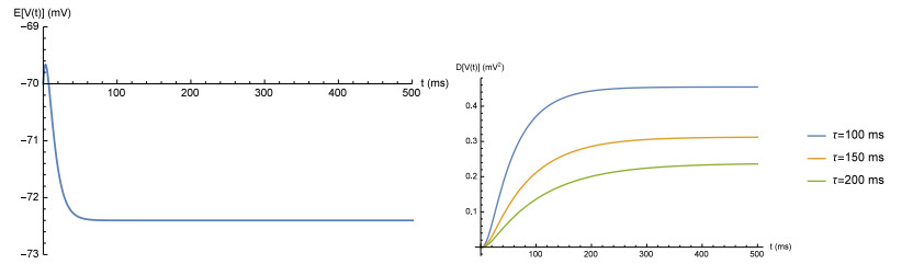
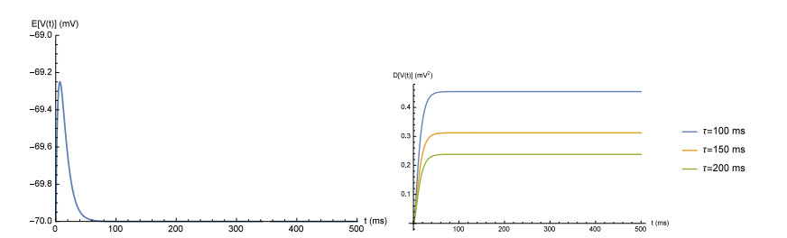
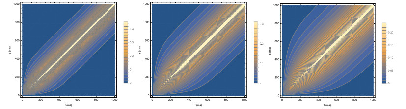
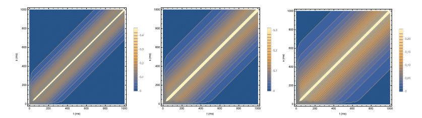
Figures(6)  /  Tables(2)

Other Articles By Authors

/

DownLoad:  Full-Size Img  PowerPoint
Return
Return

Catalog