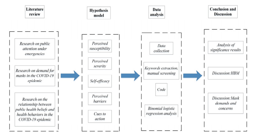
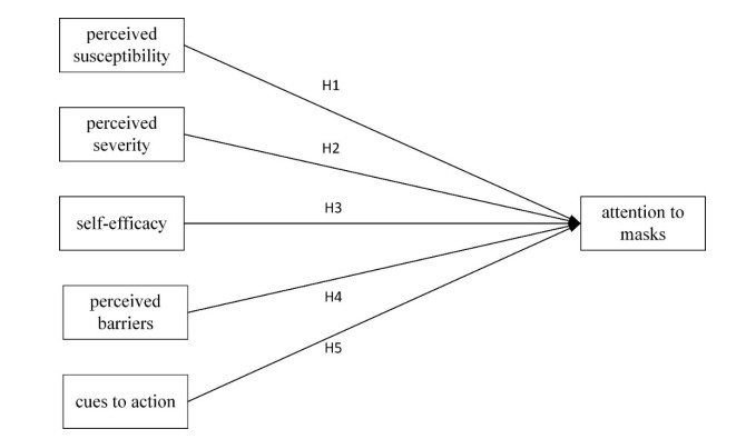
As we all know, vaccination still does not protect people from novel coronavirus infections, and wearing masks remains essential. Research on mask attention is helpful to understand the public's cognition and willingness to wear masks, but there are few studies on mask attention in the existing literature. The health belief model used to study disease prevention behaviors is rarely applied to the research on mask attention, and the research on health belief models basically entails the use of a questionnaire survey. This study was purposed to establish a health belief model affecting mask attention to explore the relationship between perceived susceptibility, perceived severity, self-efficacy, perceived impairment, action cues and mask attention. On the basis of the establishment of the hypothesis model, the Baidu index of epidemic and mask attention, the number of likes and comments on Weibo, and the historical weather temperature data were retrieved by using software. Keyword extraction and manual screening were carried out for Weibo comments, and then the independent variables and dependent variables were coded. Finally, through binomial logistic regression analysis, it was concluded that perceived susceptibility, perceived severity and action cues have significant influences on mask attention, and that the accuracy rate for predicting low attention is 93.4%, and the global accuracy is 84.3%. These conclusions can also help suppliers make production decisions.
Citation: Wei Hong, Xinhang Lu, Linhai Wu, Xujin Pu. Analysis of factors influencing public attention to masks during the COVID-19 epidemic—Data from Sina Weibo[J]. Mathematical Biosciences and Engineering, 2022, 19(7): 6469-6488. doi: 10.3934/mbe.2022304
As we all know, vaccination still does not protect people from novel coronavirus infections, and wearing masks remains essential. Research on mask attention is helpful to understand the public's cognition and willingness to wear masks, but there are few studies on mask attention in the existing literature. The health belief model used to study disease prevention behaviors is rarely applied to the research on mask attention, and the research on health belief models basically entails the use of a questionnaire survey. This study was purposed to establish a health belief model affecting mask attention to explore the relationship between perceived susceptibility, perceived severity, self-efficacy, perceived impairment, action cues and mask attention. On the basis of the establishment of the hypothesis model, the Baidu index of epidemic and mask attention, the number of likes and comments on Weibo, and the historical weather temperature data were retrieved by using software. Keyword extraction and manual screening were carried out for Weibo comments, and then the independent variables and dependent variables were coded. Finally, through binomial logistic regression analysis, it was concluded that perceived susceptibility, perceived severity and action cues have significant influences on mask attention, and that the accuracy rate for predicting low attention is 93.4%, and the global accuracy is 84.3%. These conclusions can also help suppliers make production decisions.

| [1] |
A. Remuzzi, G. Remuzzi, COVID-19 and Italy: What next? Lancet, 395 (2020), 1225-1228. https://doi.org/10.1016/S0140-6736(20)30627-9 doi: 10.1016/S0140-6736(20)30627-9

|
| [2] | World Health Organization, WHO Director General's Statement on IHR Emergency Committee on Novel Coronavirus (2019-nCoV), 2021. Available from: https://www.sunupauto.com/114755.html. |
| [3] | World Health Organization, Coronavirus Disease (COVID-19) Dashboard, 2021. Available from: https://covid19.who.int. |
| [4] |
A. Barnawi, P. Chhikara, R. Tekchandani, N. Kumar, B. Alzahrani, Artificial intelligence-enabled Internet of Things-based system for COVID-19 screening using aerial thermal imaging, Future Gener. Comput. Syst., 124 (2021), 119-132. https://doi.org/10.1016/j.future.2021.05.019 doi: 10.1016/j.future.2021.05.019
|
| [5] |
K. K. Lella, P. J. A. Alphonse, A literature review on COVID-19 disease diagnosis from respiratory sound data, AIMS Bioeng., 8 (2021), 140-153. https://doi.org/10.3934/bioeng.2021013 doi: 10.3934/bioeng.2021013
|
| [6] |
K. K. Lella, P. J. A. Alphonse, Automatic COVID-19 disease diagnosis using 1D convolutional neural network and augmentation with human respiratory sound based on parameters: Cough, breath, and voice, AIMS Public Health, 8 (2021), 240-264. https://doi.org/10.3934/publichealth.2021019 doi: 10.3934/publichealth.2021019
|
| [7] |
K. K. Lella, P. J. A. Alphonse, Automatic diagnosis of COVID-19 disease using deep convolutional neural network with multi-feature channel from respiratory sound data: Cough, voice, and breath, Alexandria Eng. J., 61 (2021), 1110-0168, https://doi.org/10.1016/j.aej.2021.06.024 doi: 10.1016/j.aej.2021.06.024
|
| [8] |
K. K. Lella, P. J. A. Alphonse, COVID-19 disease diagnosis with light-weight CNN using modified MFCC and enhanced GFCC from human respiratory sounds, Eur. Phys. J. Spec. Top., (2022), 1-18. https://doi.org/10.1140/epjs/s11734-022-00432-w doi: 10.1140/epjs/s11734-022-00432-w
|
| [9] |
A. K. Thakur, R. Sathyamurthy, R. Velraj, I. Lynch, R. Saidur, A. K. Pandey, et al., Secondary transmission of SARS-Cov-2 through wastewater: Concerns and tactics for treatment to effectively control the pandemic, J. Environ. Manage., 290 (2021), 112668. https://doi.org/10.1016/j.jenvman.2021.112668 doi: 10.1016/j.jenvman.2021.112668
|
| [10] |
J. Paananen, J. Rannikko, M. Harju, J. Pirhonen, The impact of Covid-19-related distancing on the well-being of nursing home residents and their family members: A qualitative study, Int. J. Nurs. Stud. Adv., 3 (2021), 100031. https://doi.org/10.1016/j.ijnsa.2021.100031 doi: 10.1016/j.ijnsa.2021.100031
|
| [11] |
C. Betsch, L. Korn, L. Felgendreff, S. Eitze, H. Thaiss, School opening during the SARS-CoV-2 pandemic: Public acceptance of wearing fabric masks in class, Public Health Pract., 2 (2021), 100115. https://doi.org/10.1016/j.puhip.2021.100115 doi: 10.1016/j.puhip.2021.100115
|
| [12] |
M. Shen, Z. Zeng, B. Song, H. Yi, T. Hu, Y. Zhang, et al., Neglected microplastics pollution in global COVID-19: Disposable surgical masks, Sci. Total Environ., 790 (2021), 148130. https://doi.org/10.1016/j.scitotenv.2021.148130 doi: 10.1016/j.scitotenv.2021.148130
|
| [13] |
U. A. Eke, A. C. Eke, Personal protective equipment in the siege of respiratory viral pandemics: strides made and next steps, Expert Rev. Respir. Med., 15 (2020), 441-452. https://doi.org/10.1080/17476348.2021.1865812 doi: 10.1080/17476348.2021.1865812
|
| [14] | Y. Jiang, Y. Li, Y. Zhao, Mask dilemma and innovation for production and operation mode of public health products, Sci. Res. Manage., 41 (2020), 37-46. |
| [15] |
G. Chua, K. Yuen, X. Wang, Y. Wong, The determinants of panic buying during COVID-19, Int. J. Environ. Res. Public Health , 18 (2021), 3247. https://doi.org/10.3390/ijerph18063247 doi: 10.3390/ijerph18063247
|
| [16] |
G. Tirkes, C. Guray, N. Celebi, Demand forecasting: A comparison between the Holt-Winters, trend analysis and decomposition models, Teh. Vjesn., 24 (2017), 503-509. https://doi.org/10.17559/TV-20160615204011 doi: 10.17559/TV-20160615204011
|
| [17] |
H. Yang, H. Jing, Forecasting of fresh agricultural products demand based on the ARIMA model, Guangdong Agric. Sci., 5 (2013), 855-858. https://doi.org/10.16768/j.issn.1004-874x.2013.11.001 doi: 10.16768/j.issn.1004-874x.2013.11.001
|
| [18] |
K. K. Chandriah, R. V. Naraganahalli, RNN/LSTM with modified Adam optimizer in deep learning approach for automobile spare parts demand forecasting, Multimedia Tools Appl., 80 (2021), 26145-26159. https://doi.org/10.1007/s11042-021-10913-0 doi: 10.1007/s11042-021-10913-0
|
| [19] | L. Si, Y. Wang, G. Xu, Logistics demand forecasting based on improved grey model, Comput. Simul., 29 (2012), 192-194,213. |
| [20] |
X. Xu, Y. Qi, Z. Hua, Forecasting demand of commodities after natural disasters, Expert Syst. Appl., 37 (2010), 4313-4317. https://doi.org/10.1016/j.eswa.2009.11.069 doi: 10.1016/j.eswa.2009.11.069
|
| [21] |
E. Shin, J. E. Lee, What makes consumers purchase apparel products through social shopping services that social media fashion influencers have worn, J. Bus. Res., 132 (2021), 416-428. https://doi.org/10.1016/j.jbusres.2021.04.022 doi: 10.1016/j.jbusres.2021.04.022
|
| [22] |
A. S. Al-Adwan, G. Sammour, What makes consumers purchase mobile apps: Evidence from Jordan, J. Theor. Appl. Electron. Comm., 16 (2020), 562-583. https://doi.org/10.3390/jtaer16030034 doi: 10.3390/jtaer16030034
|
| [23] | C. Li, Y. Wang, H. Qu, Study on spatial and temporal characteristics of textile intangible cultural heritage and its communication strategy: An empirical analysis based on Baidu index, J. Silk, 58 (2021), 52-58. |
| [24] |
J. Wei, W. Zhan, X. Guo, D. Marinova, Public attention to the great smog event: A case study of the 2013 smog event in Harbin, China, Nat. Hazards, 89 (2017), 923-938. https://doi.org/10.1007/s11069-017-3000-6 doi: 10.1007/s11069-017-3000-6
|
| [25] |
X. Gong, Y. Han, M. Hou, R. Guo, Online public attention during the early days of the COVID-19 pandemic: Infoveillance study based on Baidu index, JMIR Public Health Surveill., 6 (2020), 225-237. https://doi.org/10.2196/23098 doi: 10.2196/23098
|
| [26] |
Q. Feng, H. Wei, J. Hu, F. Li, P. Lv, P. Wu, Analysis of the attention to COVID-19 epidemic based on visibility graph network, Mod. Phys. Lett. B, 35 (2021), 2150316. https://doi.org/10.1142/S0217984921503164 doi: 10.1142/S0217984921503164
|
| [27] | C. Zhang, X. Ma, Y. Zhou, R. Guo, Analysis of public opinion evolution in COVID-19 pandemic from a perspective of sentiment variation, J. Geo-Inf. Sci., 23 (2021), 341-350. |
| [28] |
K. Hou, T. Hou, L. Cai, Public attention about COVID-19 on social media: An investigation based on data mining and text analysis, Pers. Individ. Differ., 175 (2021), 110701. https://doi.org/10.1016/j.paid.2021.110701 doi: 10.1016/j.paid.2021.110701
|
| [29] | Y. Zhao, S. Cheng, X. Yu, H. L. Xu, Chinese public's attention to the COVID-19 epidemic on social media: Observational descriptive study, J. Med. Internet Res., 22 (2020), e18825. http://preprints.jmir.org/preprint/18825 |
| [30] |
T. L. Phan, C. T. S. Ching, A reusable mask for coronavirus disease 2019 (COVID-19), Arch. Med. Res., 51 (2020), 455-457. https://doi.org/10.1016/j.arcmed.2020.04.001 doi: 10.1016/j.arcmed.2020.04.001
|
| [31] |
H. Wu, J. Huang, C. Zhang, Z. L. He, W. K. Ming, Facemask shortage and the novel coronavirus disease (COVID-19) outbreak: Reflections on public health measures, E Clin. Med., 21 (2020), 100329. https://doi.org/10.1016/j.eclinm.2020.100329 doi: 10.1016/j.eclinm.2020.100329
|
| [32] |
C. E. Rodriguez-Martinez, M. P. Sossa-Briceo, J. A. Cortes, Decontamination and reuse of N95 filtering facemask respirators: A systematic review of the literature, Am. J. Infect. Control, 48 (2020), 1520-1532. https://doi.org/10.1016/j.ajic.2020.07.004 doi: 10.1016/j.ajic.2020.07.004
|
| [33] |
Y. Tao, F. You, Can decontamination and reuse of N95 respirators during COVID-19 pandemic provide energy, environmental, and economic benefits? Appl. Energy, 304 (2021), 117848. https://doi.org/10.1016/j.apenergy.2021.117848 doi: 10.1016/j.apenergy.2021.117848
|
| [34] |
E. Deniz, S. Sibar, O. Kilic, S. Ayhan, Comparison of effectiveness of four facial masks used during the COVID-19 pandemic using indocyanine green and fluorescent angiography device: A plastic surgeon perspective, Turk. J. Plast. Surg., 29 (2021), 166-171. https://doi.org/10.4103/tjps.tjps_105_20 doi: 10.4103/tjps.tjps_105_20
|
| [35] | L. Wang, X. Zhao, J. Zhang, W. Ma, H. Zhao, Rational selection and application of medical masks, Chin. J. Nosocomiol., 21 (2011), 3908-3909. |
| [36] |
R. K. Goel, S. Haruna, Unmasking the demand for masks: Analytics of mandating coronavirus masks, Metroeconomica, 72 (2021), 580-591. https://doi.org/10.1111/meca.12334 doi: 10.1111/meca.12334
|
| [37] |
T. Zhang, Q. Wang, W. Shi, T. Sheng, J. X. Liu, J. J. Zhao, et al., Achieving universal wearing of face masks during the COVID-19 pandemic: A practical solution from Shanghai, China, Risk Manage. Healthcare Policy, 13 (2020), 3067-3077. https://doi.org/10.2147/RMHP.S280672 doi: 10.2147/RMHP.S280672
|
| [38] | F. J. Siyal, Z. A. Shaikh, S. Z. Ahmed, M. A. Shahid, F. Agha, M. Khoso, et al., Anxiety among COVID-19 physicians during the pandemic in the health care center of the rural region, Arch. Pharm. Pract., 11 (2020), 91-93. |
| [39] |
E. M. Kleiman, A. L. Yeager, J. L. Grove, J. K. Kellerman, J. S. Kim, Real-time mental health impact of the COVID-19 pandemic on college students: Ecological momentary assessment study, JMIR Mental Health, 7 (2020), e24815. https://doi.org/10.2196/24815 doi: 10.2196/24815
|
| [40] |
Y. P. Hsieh, C. Yen, C. Wu, P. Wang, Nonattendance at scheduled appointments in outpatient clinics due to COVID-19 and related factors in Taiwan: A health belief model approach, Int. J. Environ. Res. Public Health, 18 (2021), 4445. https://doi.org/10.3390/ijerph18094445 doi: 10.3390/ijerph18094445
|
| [41] |
C. Zhou, X. Yue, X. Zhang, F. Shangguan, X. Zhang, Self-efficacy and mental health problems during COVID-19 pandemic: A multiple mediation model based on health belief model, Pers. Individ. Differ., 179 (2021), 110893. https://doi.org/10.1016/j.paid.2021.110893 doi: 10.1016/j.paid.2021.110893
|
| [42] |
M. Aval, A. Ansari-Moghadam, G. Masoudy, Educational intervention based on health belief model on the adoption of preventive behaviors of Crimean-Congo hemorrhagic fever in ranchers, Health Scope, 8 (2019), e14112. https://doi.org/10.5812/jhealthscope.14112 doi: 10.5812/jhealthscope.14112
|
| [43] |
L. E. Bechard, M. Bergelt, B. Neudorf, T. C. DeSouza, L. E. Middleton, Using the health belief model to understand age differences in perceptions and responses to the COVID-19 pandemic, Front. Psychol., 12 (2021), 609893. https://doi.org/10.3389/fpsyg.2021.609893 doi: 10.3389/fpsyg.2021.609893
|
| [44] |
A. B. Coe, M. H. Elliott, S. B. S. Gatewood, J. R. Goode, L. R. Moczygemba, Perceptions and predictors of intention to receive the COVID-19 vaccine, Res. Soc. Adm. Pharm., 18 (2021), 2593-2599. https://doi.org/10.1016/j.sapharm.2021.04.023 doi: 10.1016/j.sapharm.2021.04.023
|
| [45] |
A. R. Mercadante, A. V. Law, Will they, or won't they? Examining patients' vaccine intention for flu and COVID-19 using the health belief model, Res. Soc. Adm. Pharm., 17 (2020), 1596-1605. https://doi.org/10.1016/j.sapharm.2020.12.012 doi: 10.1016/j.sapharm.2020.12.012
|
| [46] |
S. G. Tan, A. S. Raamkumar, H. L. Wee, Users' beliefs toward physical distancing in Facebook pages of public health authorities during COVID-19 pandemic in early 2020, Health Educ. Behav., 48 (2021), 404-411. https://doi.org/10.1177/10901981211014428 doi: 10.1177/10901981211014428
|
| [47] | N. Li, Z. Tang, Cognition and demand for health education of rural residents for public health emergencies and common infectious diseases, J. Catastrophology, 35 (2020), 33-37. |
| [48] | J. Cao, X. Yang, S. Wang, Key scientific problems in public emergency management, J. Public Manage., 4 (2007), 84-93. |
| [49] |
J. Dono, K. Ettridge, M. Wakefield, S. Pettigrew, J. Coveney, D. Roder, et al., Intentions to reduce sugar-sweetened beverage consumption: The importance of perceived susceptibility to health risks, Public Health Nutr., 24 (2021), 5663-5672. https://doi.org/10.1017/S1368980021000239 doi: 10.1017/S1368980021000239
|
| [50] |
J. Joo, Exploration of structural relations on health behavior related to particulate matter: Focused on multi-dimensional health locus of control, perceived susceptibility and severity, and health behavioral intention, J. Korea Convergence Soc., 8 (2017), 413-421. https://doi.org/10.15207/JKCS.2017.8.11.413 doi: 10.15207/JKCS.2017.8.11.413
|
| [51] |
A. Almehmadi, COVID-19 pandemic data predict the stock market, Comput. Syst. Sci. Eng., 36 (2021), 451-460. https://doi.org/10.32604/csse.2021.015309 doi: 10.32604/csse.2021.015309
|
| [52] |
M. Wang, L. Huang, X. Liang, B. Li, Consumer knowledge, risk perception and food-handling behaviors—A national survey in China, Food Control, 122 (2021), 107789. https://doi.org/10.1016/j.foodcont.2020.107789 doi: 10.1016/j.foodcont.2020.107789
|
| [53] |
J. L. Marle, F. Parmentier, F. Vinchon, M. Torme, X. Borteyrou, T. Lubart, Evolution and impact of self-efficacy during French COVID-19 confinement: A longitudinal study, J. Gen. Physiol., 148 (2021), 360-381. https://doi.org/10.1080/00221309.2021.1904815 doi: 10.1080/00221309.2021.1904815
|
| [54] |
H. T. Duong, H. T. Nguyen, S. J. Mcfarlane, L. T. V. Nguyen, Risk perception and COVID-19 preventive behaviors: Application of the integrative model of behavioral prediction, Soc. Sci. J., (2021), 1-14. https://doi.org/10.1080/03623319.2021.1874176 doi: 10.1080/03623319.2021.1874176
|
| [55] |
M. Morishima, K. Kishida, M. Fukagawa, Investigating facemask problems associated with wearing comfort and fit, Int. J. Clothing Sci. Technol., (2021). https://doi.org/10.1108/IJCST-05-2020-0067 doi: 10.1108/IJCST-05-2020-0067
|
| [56] |
Y. Lin, C. Chen, Thermoregulation and thermal sensation in response to wearing tight-fitting respirators and exercising in hot-and-humid indoor environment, Build. Environ., 160 (2019), 106158. https://doi.org/10.1016/j.buildenv.2019.05.036 doi: 10.1016/j.buildenv.2019.05.036
|
| [57] |
A. A. Sadore, D. W. Handiso, T. E. Wontamo, D. E. Mekango, S. Moges, Influence of social media use on practice of Covid-19 preventive measures among Ethiopian residents: An online cross-sectional study, Disaster Med. Public, (2021), 1-6. https://doi.org/10.1017/dmp.2021.184 doi: 10.1017/dmp.2021.184
|
| [58] | E. Kendal, Public health crises in popular media: How viral outbreak films affect the public's health literacy, Med. Humanit., 47 (2019), 11-19. https://10.1136/medhum-2018-011446 |
| [59] |
Y. Ye, R. Wang, D. Feng, R. J. Wu, Z. F. Li, C. X. Long, et al., The recommended and excessive preventive behaviors during the COVID-19 pandemic: A community-based online survey in China, Int. J. Environ. Res. Public Health, 17 (2020), 6953. https://doi.org/10.3390/ijerph17196953 doi: 10.3390/ijerph17196953
|
| [60] |
Z. Liu, T. Huynh, P. Dai, The impact of COVID-19 on the stock market crash risk in China, Res. Int. Bus. Finance, 57 (2021), 101419. https://doi.org/10.1016/j.ribaf.2021.101419 doi: 10.1016/j.ribaf.2021.101419
|
| [61] |
X. Zhu, C. Xia, Visual network analysis of the Baidu-index data on greenhouse gas, Int. J. Mod. Phys. B, 35 (2021), 2150115. https://doi.org/10.1142/S0217979221501150 doi: 10.1142/S0217979221501150
|
| [62] |
Y. Yuan, X. Wang, Exploring the effectiveness of location-based social media in modeling user activity space: A case study of Weibo, Trans. GIS., 22 (2018), 930-957. https://doi.org/10.1111/tgis.12450 doi: 10.1111/tgis.12450
|
| [63] |
T. Kawada, Indices of insulin sensitivity and resistance: Adequate logarithmic transformation is needed to keep mathematical equivalence, Early Hum. Dev., 89 (2013), 515. https://doi.org/10.1016/j.earlhumdev.2013.03.010 doi: 10.1016/j.earlhumdev.2013.03.010
|
| [64] |
R. Zhang, J. Liu, L. Zhang, J. D. Lin, Q. Q. Wu, The distorted power of medical surgical masks for changing the human thermal psychology of indoor personnel in summer, Indoor Air, 31 (2021), 1645-1656. https://doi.org/10.1111/ina.12830 doi: 10.1111/ina.12830
|
| [65] |
R. Johnston, K. Jones, D. Manley, Confounding and collinearity in regression analysis: A cautionary tale and an alternative procedure, illustrated by studies of British voting behaviour, Qual. Quant., 52 (2018), 1957-1976. https://doi.org/10.1007/s11135-017-0584-6 doi: 10.1007/s11135-017-0584-6
|
| [66] |
T. J. Wang, H. J. Wang, Y. J. Zeng, X. Q. Cai, L. D. Xie, Health beliefs associated with preventive behaviors against non-communicable diseases, Patient Educ. Couns., 105 (2022), 173-181. https://doi.org/10.1016/j.pec.2021.05.024 doi: 10.1016/j.pec.2021.05.024
|
Figures(2) / Tables(8)

Wei Hong, Xinhang Lu, Linhai Wu, Xujin Pu. Analysis of factors influencing public attention to masks during the COVID-19 epidemic—Data from Sina Weibo[J]. Mathematical Biosciences and Engineering, 2022, 19(7): 6469-6488. doi: 10.3934/mbe.2022304


 DownLoad: