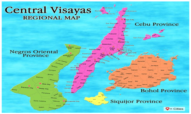
The pandemic has underscored the importance of the environment. In this study, the environmental condition of Central Visayas, Philippines has been assessed and evaluated before and during the onset of the COVID-19 pandemic to deal with a possible association between the environmental indicators and the pandemic. The relationships between environmental key variables namely: air quality, air pollution, water quality, water pollution, and solid waste management have been quantified. The study utilized secondary data sources from a review of records from government agencies and LGUs in Region 7. This study also provides a framework which is the pandemics and epidemics in environmental aspects. The paper concludes by offering researchers and policymakers to promote changes in environmental policies and provide some recommendations for adequately controlling future pandemic and epidemic threats in Central Visayas, Philippines.
Citation: Clare Maristela V. Galon, James G. Esguerra. Impact of COVID-19 on the environment sector: a case study of Central Visayas, Philippines[J]. AIMS Environmental Science, 2022, 9(2): 106-121. doi: 10.3934/environsci.2022008
The pandemic has underscored the importance of the environment. In this study, the environmental condition of Central Visayas, Philippines has been assessed and evaluated before and during the onset of the COVID-19 pandemic to deal with a possible association between the environmental indicators and the pandemic. The relationships between environmental key variables namely: air quality, air pollution, water quality, water pollution, and solid waste management have been quantified. The study utilized secondary data sources from a review of records from government agencies and LGUs in Region 7. This study also provides a framework which is the pandemics and epidemics in environmental aspects. The paper concludes by offering researchers and policymakers to promote changes in environmental policies and provide some recommendations for adequately controlling future pandemic and epidemic threats in Central Visayas, Philippines.

| [1] | World Health Organization. (2020). Transmission of SARS-COV-2: Implications for infection prevention precautions. World Health Organization. Retrieved February 16, 2022, from https://www.who.int/news-room/commentaries/detail/transmission-of-sars-cov-2-implications-for-infection-prevention-precautions |
| [2] |
Deress T, Hassen F, Adane K, et al (2018). Assessment of knowledge, attitude, and practice about biomedical waste management and associated factors among the healthcare professionals at Debre Markos Town Healthcare facilities, Northwest Ethiopia. J Environ Public Health 2018: 7672981. https://doi.org/10.1155/2018/7672981 doi: 10.1155/2018/7672981

|
| [3] | Santamouris M, Kolokotsa D (2016). URBAN CLIMATE MITIGATION TECHNIQUES. Routledge |
| [4] |
Bala BK, Arshad M, Noh KM. (2016). Modelling of solid waste management systems of Dhaka City in Bangladesh. Springer Texts Bus Econ 249–274. https://doi.org/10.1007/978-981-10-2045-2_12 doi: 10.1007/978-981-10-2045-2_12
|
| [5] |
Arbulú I, Lozano J, Rey-Maquieira J. (2016). The challenges of municipal solid waste management systems provided by public-private partnerships in mature tourist destinations: The case of Mallorca. Waste Manage 51: 252–258. doi: 10.1016/j.wasman.2016.03.007
|
| [6] |
Houessionon MG, Ouendo EMD, Bouland C, et al. (2021). Environmental heavy metal contamination from Electronic Waste (e-waste) recycling activities worldwide: A systematic review from 2005 to 2017. Int J Environ Res Pub He 18: 3517. https://doi.org/10.3390/ijerph18073517 doi: 10.3390/ijerph18073517
|
| [7] |
Theunis J, Stevens M, Botteldooren D (2016). Sensing the environment. Und Com Sys 21–46. https://doi.org/10.1007/978-3-319-25658-0_2 doi: 10.1007/978-3-319-25658-0_2
|
| [8] |
Zhu Z, Chen B, Zhao Y, et al (2021). Multi-sensing paradigm based urban air quality monitoring and hazardous gas source analyzing: A Review. J Saf Sci Rese 2: 131–145. https://doi.org/10.1016/j.jnlssr.2021.08.004 doi: 10.1016/j.jnlssr.2021.08.004
|
| [9] | Almaden C R C (2014). Protecting the water supply: The Philippine experience. J Soc Polit Econ Stud 39: 467–49 |
| [10] |
Bashir M F, Jiang B, Komal B, et al. (2020). Correlation between environmental pollution indicators and COVID-19 pandemic: A brief study in Californian context. Environ Res 187: 109652. https://doi.org/10.1016/j.envres.2020.109652 doi: 10.1016/j.envres.2020.109652
|
| [11] |
Xu K, Cui K, Young L H, et al. (2020). Impact of the COVID-19 event on air quality in Central China. Aerosol and Air Qual Res 20: 915–929. https://doi.org/10.4209/aaqr.2020.04.0150 doi: 10.4209/aaqr.2020.04.0150
|
| [12] | United Nations (2014) World Urbanization Prospects: The 2014 Revision, Highlights. New York: Department of Economic and Social Affairs, Population Division, United Nations. |
| [13] |
Atta U, Hussain M, Malik R N (2020). Environmental impact assessment of municipal solid waste management value chain: A case study from Pakistan. Waste Manag Res: J Sust Circular Econ 38: 1379–1388. https://doi.org/10.1177/0734242x20942595 doi: 10.1177/0734242x20942595
|
| [14] |
Baniasad M, Mofrad M G, Bahmanabadi B, et al. (2021). Covid-19 in Asia: Transmission factors, re-opening policies, and Vaccination simulation. Environ Res 202: 111657. https://doi.org/10.1016/j.envres.2021.111657 doi: 10.1016/j.envres.2021.111657
|
| [15] |
Vasistha P, Ganguly R (2020). Water quality assessment of natural lakes and its importance: An overview. Mater Today: P 32: 544–552. https://doi.org/10.1016/j.matpr.2020.02.092 doi: 10.1016/j.matpr.2020.02.092
|
| [16] | Abbaspour S (2011). Water quality in developing countries, South Asia, South Africa, water quality management, and activities that cause water pollution. IPCBEE 15: e102 |
| [17] | Environmental Management Bureau 7, Department of Environment and Natural Resources. (2019). Regional State of the Brown Environment Report 2019. |
| [18] |
Eroğlu H (2020). Effects of covid-19 outbreak on environment and Renewable Energy Sector. Environ Dev Sustain 23: 4782–4790. https://doi.org/10.1007/s10668-020-00837-4 doi: 10.1007/s10668-020-00837-4
|
| [19] |
Shakil M H, Munim Z H, Tasnia M, et al. (2020). Covid-19 and the environment: A critical review and research agenda. Sci Total Environ 745: 141022. https://doi.org/10.1016/j.scitotenv.2020.141022 doi: 10.1016/j.scitotenv.2020.141022
|
| [20] | Environmental Management Bureau 7, Department of Environment and Natural Resources. (2019). Regional State of the Brown Environment Report 2019. |
| [21] | Environmental Management Bureau 7, Department of Environment and Natural Resources. (2019). Regional State of the Brown Environment Report 2020 |
| [22] |
Chirani M R, Kowsari E, Teymourian T, et al. (2021). Environmental impact of increased soap consumption during COVID-19 pandemic: Biodegradable soap production and sustainable packaging. Sci Total Environ 796: 149013. https://doi.org/10.1016/j.scitotenv.2021.149013 doi: 10.1016/j.scitotenv.2021.149013
|
| [23] |
Santos G D (2021). 2020 tropical cyclones in the Philippines: A Review. Trop Cyclone Res Rev 10: 191–199. https://doi.org/10.1016/j.tcrr.2021.09.003 doi: 10.1016/j.tcrr.2021.09.003
|
| [24] |
Rume T, Islam SU. (2020). Environmental effects of COVID-19 pandemic and potential strategies of sustainability. Heliyon 6: e04965. doi: 10.1016/j.heliyon.2020.e04965
|
| [25] |
Ncube LK, Ude AU, Ogunmuyiwa EN, et al. (2021). An overview of plastic waste generation and management in food packaging industries. Recycling 6: 12. https://doi.org/10.3390/recycling6010012 doi: 10.3390/recycling6010012
|
 Environ-09-02-08-s1.pdf Environ-09-02-08-s1.pdf |
 |
Figures(8) / Tables(8)

Clare Maristela V. Galon, James G. Esguerra. Impact of COVID-19 on the environment sector: a case study of Central Visayas, Philippines[J]. AIMS Environmental Science, 2022, 9(2): 106-121. doi: 10.3934/environsci.2022008


 DownLoad: