In this work, we report a large-scale synchronized replacement pattern of the Alpha (B.1.1.7) variant by the Delta (B.1.617.2) variant of SARS-COV-2. We argue that this phenomenon is associated with the invasion timing and the transmissibility advantage of the Delta (B.1.617.2) variant. Alpha (B.1.1.7) variant skipped some countries/regions, e.g. India and neighboring countries/regions, which could have led to a mild first wave before the invasion of the Delta (B.1.617.2) variant, in term of reported COVID-deaths per capita.
Citation: Yuan Liu, Anyin Feng, Shi Zhao, Weiming Wang, Daihai He. Large-scale synchronized replacement of Alpha (B.1.1.7) variant by the Delta (B.1.617.2) variant of SARS-COV-2 in the COVID-19 pandemic[J]. Mathematical Biosciences and Engineering, 2022, 19(4): 3591-3596. doi: 10.3934/mbe.2022165
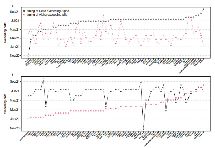
In this work, we report a large-scale synchronized replacement pattern of the Alpha (B.1.1.7) variant by the Delta (B.1.617.2) variant of SARS-COV-2. We argue that this phenomenon is associated with the invasion timing and the transmissibility advantage of the Delta (B.1.617.2) variant. Alpha (B.1.1.7) variant skipped some countries/regions, e.g. India and neighboring countries/regions, which could have led to a mild first wave before the invasion of the Delta (B.1.617.2) variant, in term of reported COVID-deaths per capita.

| [1] |
C. Wang, Z. Wang, G. Wang, J. Y. N. Lau, K. Zhang, W. Li, COVID-19 in early 2021: Current status and looking forward, Sig. Transduct Targeted Ther., 6 (2021), 1–14. http://doi.org/10.038/s41392-021-00527-1 doi: 10.038/s41392-021-00527-1

|
| [2] |
T. Chookajorn, T. Kochakarn, C. Wilasang, N. Kotanan, C. Modchang, Southeast Asia is an emerging hotspot for COVID-19, Nat Med., 27 (2021), 1495–1496. https://doi.org/10.1038/s41591-021-01471-x doi: 10.1038/s41591-021-01471-x
|
| [3] |
M. Vassallo, S. Manni, C. Klotz C, et al., Patients admitted for variant alpha COVID-19 have poorer outcomes than those infected with the old strain, J. Clin. Med., 10 (2021), 3550. https://doi.org/10.3390/jcm10163550 doi: 10.3390/jcm10163550
|
| [4] |
T. Farinholt, H. Doddapaneni, X. Qin, et al., Transmission event of SARS-CoV-2 Delta variant reveals multiple vaccine breakthrough infections, BMC Med., 19 (2021), 1–6. https://doi.org/10.1186/s12916-021-02103-4 doi: 10.1186/s12916-021-02103-4
|
| [5] |
Y. Liu, A. A. Gayle, A. Wilder-Smith, J. Rocklöv, The reproductive number of COVID-19 is higher compared to SARS coronavirus, J. Travel Med., 27 (2020), taaa021. https://doi.org/10.1093/jtm/taaa021 doi: 10.1093/jtm/taaa021
|
| [6] |
Y. Liu, J. Liu, K. S. Plante, J. A. Plante, X. P. Xie, X. W. Zhang, et al., The N501Y spike substitution enhances SARS-CoV-2 infection and transmission, Nature, (2021), 1–9. https://doi.org/10.1038/s41586-021-04245-0 doi: 10.1038/s41586-021-04245-0
|
| [7] |
O. Mor, M. Mandelboim, S. Fleishon, E. Bucris, D. Bar-Ilan, M. Linial, et al., The rise and fall of a local SARS-CoV-2 variant with the spike protein mutation L452R, Vaccines, 9 (2021), 937. https://doi.org/10.3390/vaccines9080937 doi: 10.3390/vaccines9080937
|
| [8] |
S. Shiehzadegan, N. Alaghemand, M. Fox, V. Venketaraman, Analysis of the delta variant B. 1.617. 2 COVID-19, Clin. Pract., 11 (2021), 778–784. https://doi.org/10.3390/clinpract11040093 doi: 10.3390/clinpract11040093
|
| [9] |
N. Ghosh, I. Saha, J. P. Sarkar, U. Maulik, Strategies for COVID-19 epidemiological surveillance in India: overall policies till June 2021, Frontiers Public Health, 9 (2021). https://doi.org/10.3389/fpubh.2021.708224 doi: 10.3389/fpubh.2021.708224
|
| [10] |
S. Shrivastava, S. T. Mhaske, M. S. Modak, R. G. Virkar, S. S. Pisal, A. C. Mishra, et al., Emergence of two distinct variants of SARS-CoV-2 and explosive second wave of COVID-19: An experience from a tertiary care hospital, Pune, India, Arch. Virol., (2022), 1–11. https://doi.org/10.1007/s00705-021-05320-7 doi: 10.1007/s00705-021-05320-7
|
| [11] |
S. Khare, C. Gurry, L. Freitas, M. B. Schultz, G.Bach, A. Diallo, et al., GISAID's role in pandemic response, China CDC Weekly, 3 (2021), 1049. https://doi.org/10.46234/ccdcw2021.255 doi: 10.46234/ccdcw2021.255
|
| [12] |
S. Elbe, G. Buckland-Merrett, Data, disease and diplomacy: GISAID's innovative contribution to global health, Global challenges, 1 (2017), 33–46. https://doi.org/10.1002/gch2.1018 doi: 10.1002/gch2.1018
|
| [13] |
Y. Shu, J. McCauley, GISAID: Global intiative on sharing all influenza data—from vision to reality, Euro. surveill., 22 (2017). https://doi.org/10.2807/1560-7917.ES.2017.22.13.30494 doi: 10.2807/1560-7917.ES.2017.22.13.30494
|
| [14] |
S. Reardon, How the Delta variant achieves its ultrafast spread, Nature, 21 (2021). https://doi.org/10.1038/d41586-021-01986-w doi: 10.1038/d41586-021-01986-w
|
| [15] |
M. Cevik, N. D. Grubaugh, A. Iwasaki, P. Openshaw, COVID-19 vaccines: Keeping pace with SARS-CoV-2 variants, Cell, 184 (2021), 5077–5081. https://doi.org/10.1016/j.cell.2021.09.010 doi: 10.1016/j.cell.2021.09.010
|
| [16] |
P. Rohani, D. J. Earn, B. T. Grenfell, Opposite patterns of synchrony in sympatric disease metapopulations, Science, 286 (1999), 968–971. https://doi.org/10.1126/science.286.5441.968 doi: 10.1126/science.286.5441.968
|
| [17] |
P. Rohani, C. Green, N. Mantilla-Beniers, B. Grenfell, Ecological interference between fatal diseases, Nature, 422 (2003), 885–888. https://doi.org/10.1038/nature01542 doi: 10.1038/nature01542
|

Figures(2)

Yuan Liu, Anyin Feng, Shi Zhao, Weiming Wang, Daihai He. Large-scale synchronized replacement of Alpha (B.1.1.7) variant by the Delta (B.1.617.2) variant of SARS-COV-2 in the COVID-19 pandemic[J]. Mathematical Biosciences and Engineering, 2022, 19(4): 3591-3596. doi: 10.3934/mbe.2022165


 DownLoad: