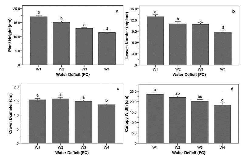
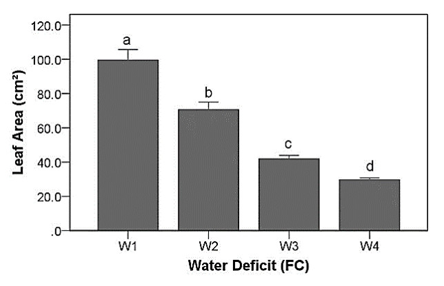
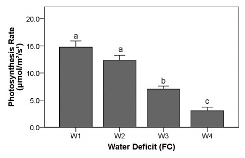
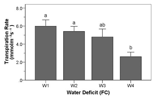
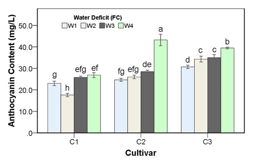
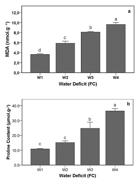
Drought stress is one of the challenges that can affect the growth and the quality of strawberry. The study aims to determine the growth, biochemical changes and leaf gas exchange of three strawberry cultivars under drought stress. This study was conducted in a glasshouse at Indonesian Citrus and Subtropical Fruits Research Institute, Indonesia, from July-November 2018. The experiment was arranged in a factorial randomized completely block design (RCBD) with three replications and four water deficit (WD) levels [100% field capacity (FC)/well-watered), 75% of FC (mild WD), 50% of FC (moderate WD), and 25% of FC (severe WD)] for three strawberry cultivars (Earlibrite, California and Sweet Charlie). The results showed that total chlorophyll and anthocyanin contents (p ≤ 0.05) were influenced by the interaction effects of cultivars and water deficit. Whereas other parameters such as plant growth, transpiration rate (E), net photosynthesis (A), stomatal conductance (gs), leaf relative water content (LRWC), flowers and fruits numbers, proline content, length, diameter, weight and total soluble solid (TSS) of fruit were affected by water deficit. A had positive significant correlation with plant height (r = 0.808), leaf area (r = 0.777), fruit length (r = 0.906), fruit diameter (r = 0.889) and fruit weight (r = 0.891). Based on the results, cultivars affected LRWC, and also number of flowers and fruits of the strawberry. This study showed that water deficit decreased plant growth, chlorophyll content, leaf gas exchange, leaf relative water content, length, diameter and weight of fruit but enhanced TSS, anthocyanin, MDA, and proline contents. Increased anthocyanin and proline contents are mechanisms for protecting plants against the effects of water stress. California strawberry had the highest numbers of flowers and fruits, and also anthocyanin content. Hence, this cultivar is recommended to be planted under drought stress conditions. Among all water stress treatments, 75% of FC had the best results to optimize water utilization on the strawberry plants.
Citation: Yenni, Mohd Hafiz Ibrahim, Rosimah Nulit, Siti Zaharah Sakimin. Influence of drought stress on growth, biochemical changes and leaf gas exchange of strawberry (Fragaria × ananassa Duch.) in Indonesia[J]. AIMS Agriculture and Food, 2022, 7(1): 37-60. doi: 10.3934/agrfood.2022003
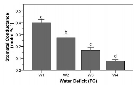
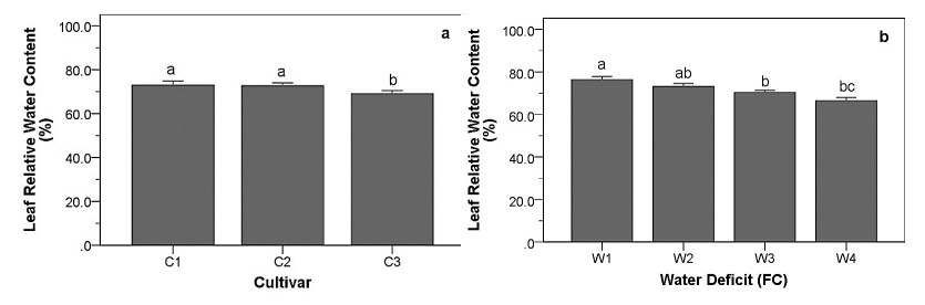
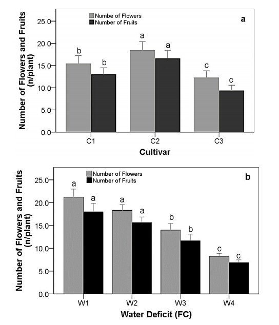
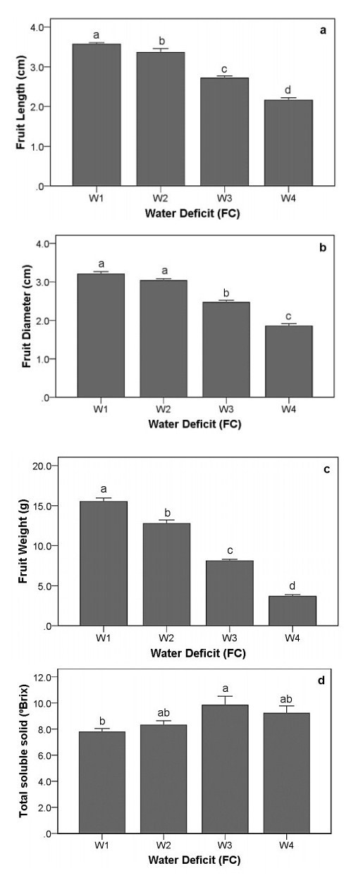
Drought stress is one of the challenges that can affect the growth and the quality of strawberry. The study aims to determine the growth, biochemical changes and leaf gas exchange of three strawberry cultivars under drought stress. This study was conducted in a glasshouse at Indonesian Citrus and Subtropical Fruits Research Institute, Indonesia, from July-November 2018. The experiment was arranged in a factorial randomized completely block design (RCBD) with three replications and four water deficit (WD) levels [100% field capacity (FC)/well-watered), 75% of FC (mild WD), 50% of FC (moderate WD), and 25% of FC (severe WD)] for three strawberry cultivars (Earlibrite, California and Sweet Charlie). The results showed that total chlorophyll and anthocyanin contents (p ≤ 0.05) were influenced by the interaction effects of cultivars and water deficit. Whereas other parameters such as plant growth, transpiration rate (E), net photosynthesis (A), stomatal conductance (gs), leaf relative water content (LRWC), flowers and fruits numbers, proline content, length, diameter, weight and total soluble solid (TSS) of fruit were affected by water deficit. A had positive significant correlation with plant height (r = 0.808), leaf area (r = 0.777), fruit length (r = 0.906), fruit diameter (r = 0.889) and fruit weight (r = 0.891). Based on the results, cultivars affected LRWC, and also number of flowers and fruits of the strawberry. This study showed that water deficit decreased plant growth, chlorophyll content, leaf gas exchange, leaf relative water content, length, diameter and weight of fruit but enhanced TSS, anthocyanin, MDA, and proline contents. Increased anthocyanin and proline contents are mechanisms for protecting plants against the effects of water stress. California strawberry had the highest numbers of flowers and fruits, and also anthocyanin content. Hence, this cultivar is recommended to be planted under drought stress conditions. Among all water stress treatments, 75% of FC had the best results to optimize water utilization on the strawberry plants.

| [1] |
Galli V, da Silva Messias R, Perin E C, et al. (2016) Mild salt stress improves strawberry fruit quality. LWT-Food Sci Technol 73: 693–699. https://doi.org/10.1016/j.lwt.2016.07.001 doi: 10.1016/j.lwt.2016.07.001

|
| [2] |
Giamperi F, Tulipani S, Alvarez-Suarez JM, et al. (2012) The strawberry: Composition, nutritional quality, and impact on human health. Nutrition 28: 9–19. https://doi.org/10.1016/j.nut.2011.08.009 doi: 10.1016/j.nut.2011.08.009
|
| [3] | Hanif Z, Ashari H (2013) Strawberry (Fragaria x ananassa) spread areas in Indonesia. In: Applying technology innovation in supporting competitive and diversified horticulture development based on local resources, Proceedings of National Seminar Book 1, Lembang July 5, 2012: Indonesian centre for Horticulture Research and Development, 87–95. |
| [4] |
Kannaujia PK, Asrey A, Bhatia K, et al. (2014) Cultivars and sequential harvesting influence physiological and functional quality of strawberry fruits. Fruits 69: 239–246. https://doi.org/10.1051/fruits/2014013 doi: 10.1051/fruits/2014013
|
| [5] |
Chaves MM, Flexas J, Pinheiro C (2009) Photosynthesis under drought and salt stress: Regulation mechanisms from whole plant to cell. Ann. Bot 103: 551–560. https://doi.org/10.1093/aob/mcn125 doi: 10.1093/aob/mcn125
|
| [6] |
Flexas J, Medrano H (2002) Drought-inhibition of photosynthesis in C3 plants : Stomatal and non-stomatal limitations revisited. Ann Bot 89: 183–189. https://doi.org/10.1093/aob/mcf027 doi: 10.1093/aob/mcf027
|
| [7] | Klamkowski K, Treder W, Wojcik K (2015) Effects of long-term water stress on leaf gas exchange, growth and yield of three strawberry cultivars. Acta Sci Pol Hortorum Cultus 14: 55–65. |
| [8] | Klamkowski K, Treder W (2006) Morphological and physiological responses of strawberry plants to water stress. Agric Conspec Sci 71: 159–165. |
| [9] |
Boyer JS (1982) Plant Productivity and Enviroment. Science 218: 443–448. https://doi.org/10.1126/science.218.4571.443 doi: 10.1126/science.218.4571.443
|
| [10] |
Gehrmann H (1985) Growth, yield and fruit quality of strawberries as affected by water supply. Acta Hortic 171: 463–469. https://doi.org/10.17660/ActaHortic.1985.171.44 doi: 10.17660/ActaHortic.1985.171.44
|
| [11] | Nezhadahmadi A, Faruq G, Rashid K (2015) The impact of drought stress on morphological and physiological parameters of three strawberry varieties in different growing conditions. Pakistan J Agric Sci 52: 79–92. |
| [12] |
Rizza F, Badeck FW, Cattivelli L, et al. (2004) Use of a water stress index to identify barley genotypes adapted to rainfed and irrigated conditions. Crop Sci Soc Am 44: 2127–2137. https://doi.org/10.2135/cropsci2004.2127 doi: 10.2135/cropsci2004.2127
|
| [13] |
Singer SM, Helmy YI, Karas AN, et al. (2003) Influences of different water-stress treatments on growth, development and production of snap bean (Phaseolus vulgaris L.). Acta Hor 614: 605–611. https://doi.org/10.17660/ActaHortic.2003.614.90 doi: 10.17660/ActaHortic.2003.614.90
|
| [14] |
Dehghanipoodeh S, Ghobadi C, Baninasab B, et al. (2018) Effect of silicon on growth and development of strawberry under water deficit conditions. Hortic Plant J 4: 226–232. https://doi.org/10.1016/j.hpj.2018.09.004 doi: 10.1016/j.hpj.2018.09.004
|
| [15] |
Adak N, Gubbuk H, Tetik N (2018) Yield, quality and biochemical properties of various strawberry cultivars under water stress. J Sci Food Agric 98: 304–311. https://doi.org/10.1002/jsfa.8471 doi: 10.1002/jsfa.8471
|
| [16] |
Bano N, Qureshi KM (2017) Responses of strawberry plant to pre-harvest application of salicylic acid in drought conditions. Pakistan J Agric Res 30: 272–286. https://doi.org/10.17582/journal.pjar/2017.30.3.272.286 doi: 10.17582/journal.pjar/2017.30.3.272.286
|
| [17] | Zaimah F, Prihastanti E, Haryati S (2013) The influence of cutting time of strawberry runners to strawberry growth (Fragaria vesca L.). Bul Anat Physiol XXI: 9–20. |
| [18] |
Zhang Z, Tian F, Hu H, et al. (2014) A comparison of methods for determining field evapotranspiration: Photosynthesis system, sap flow, and eddy covariance. Hydrol Earth Syst Sci 18: 1053–1072. https://doi.org/10.5194/hess-18-1053-2014 doi: 10.5194/hess-18-1053-2014
|
| [19] |
Barrs HD, Weatherley PE (1962) A re-examination of the relative turgidity technique for estimating water deficits in leaves. Aust J Biol Sci 15:413–428. https://doi.org/10.1071/BI9620413 doi: 10.1071/BI9620413
|
| [20] |
Ncama K, Opara UL, Tesfay SZ, et al. (2017) Application of Vis/NIR spectroscopy for predicting sweetness and flavour parameters of "Valencia" orange (Citrus sinensis) and "Star Ruby" grapefruit (Citrus x paradisi Macfad). J Food Eng 193: 86–94. https://doi.org/10.1016/j.jfoodeng.2016.08.015 doi: 10.1016/j.jfoodeng.2016.08.015
|
| [21] |
Wintermans JFGA, de Mots A (1965) Spectrophotometric characteristic of chlorophyll a and b at their phenophytins in ethanol. Biochim Biophys Acta 109: 448–453. https://doi.org/10.1016/0926-6585(65)90170-6 doi: 10.1016/0926-6585(65)90170-6
|
| [22] |
Lee J, Durst RW, Wrolstad RE (2005) Determination of total monomeric anthocyanin pigment content of fruit juices, beverages, natural colorants, and wines by the pH differential method: Collaborative study. J AOAC Int 88: 1269–1278. https://doi.org/10.1093/jaoac/88.5.1269 doi: 10.1093/jaoac/88.5.1269
|
| [23] |
Dhindsa RS, Plumb-dhindsa P, Thorpe TA (1981) Leaf senescence: correlated with increased levels of membrane permeability and lipid peroxidation, and decreased levels of superoxide dismutase and catalase. J Exp Bot 32: 93–101. https://doi.org/10.1093/jxb/32.1.93 doi: 10.1093/jxb/32.1.93
|
| [24] |
Bates LS, Waldren RP, Teare ID (1973) Rapid determination of free proline for water-stress studies. Plant Soil 39: 205–7. https://doi.org/10.1007/BF00018060 doi: 10.1007/BF00018060
|
| [25] |
Boyer JS (1970) Leaf enlargement and metabolic rates in corn, soybean, and sunflower at various leaf water potentials. Plant Physiol 46: 233–5. https://doi.org/10.1104/pp.46.2.233 doi: 10.1104/pp.46.2.233
|
| [26] |
Hsiao TC (1973) Plant responses to water stress. Annu Rev Plant Physiol 24: 519–70. https://doi.org/10.1146/annurev.pp.24.060173.002511 doi: 10.1146/annurev.pp.24.060173.002511
|
| [27] | Lisar SYS, Motafakkerazad R, Hossain MM, et al. (2012) Water Stress in plants: Causes, effects and responses. In: Rahman IMM, Hasegawa H, (Eds.), Water Stress, Croatia: InTech, 1–14. https://doi.org/10.5772/39363 |
| [28] | Bradford KJ, Hsiao TC (1982) Physiological responses to moderate water stress. In: Encyclopedia of Plant Physiology, ed AP Gottingen and MHZ Harvard (Springer_Verlag): 262–324. https://doi.org/10.1007/978-3-642-68150-9_10 |
| [29] |
Hussain M, Malik MA, Farooq M, et al. (2008) Improving drought tolerance by exogenous application of glycinebetaine and salicylic acid in sunflower. J Agron Crop Sci 194: 193–199. https://doi.org/10.1111/j.1439-037X.2008.00305.x doi: 10.1111/j.1439-037X.2008.00305.x
|
| [30] |
Kaya MD, Okçu G, Atak M, et al. (2006) Seed treatments to overcome salt and drought stress during germination in sunflower (Helianthus annuus L.). Eur J Agron 24: 291–5. https://doi.org/10.1016/j.eja.2005.08.001 doi: 10.1016/j.eja.2005.08.001
|
| [31] |
Nonami H (1998) Plant water relations and control of cell elongation at low water potentials. J Plant Res 111: 373–382. https://doi.org/10.1007/BF02507801 doi: 10.1007/BF02507801
|
| [32] | Taiz L, Zeiger E (2010) Physiology Plants, Fifth Edition, Massachusetts U.S.A: Sinauer Associates Inc, 692. |
| [33] | Klamkowski K, Treder W (2008) Response to drought stress of three strawberry cultivars grown under greenhouse conditions. J Fruit Ornam Plant Res 16: 179–188. |
| [34] |
Rodríguez P, Torrecillas A, Morales MA, et al. (2005) Effects of NaCl salinity and water stress on growth and leaf water relations of Asteriscus maritimus plants. Environ Exp Bot 53: 113–123. https://doi.org/10.1016/j.envexpbot.2004.03.005 doi: 10.1016/j.envexpbot.2004.03.005
|
| [35] |
Shao HB, Chu LY, Jaleel CA, et al. (2008) Water-deficit stress-induced anatomical changes in higher plants. Comptes Rendus-Biol 331: 215–225. https://doi.org/10.1016/j.crvi.2008.01.002 doi: 10.1016/j.crvi.2008.01.002
|
| [36] |
Zhang X, Lei L, Lai J, et al. (2018) Effects of drought stress and water recovery on physiological responses and gene expression in maize seedlings. BMC Plant Biol 18: 1–16. https://doi.org/10.1186/s12870-018-1281-x doi: 10.1186/s12870-018-1281-x
|
| [37] |
Bloch D, Hoffmann CM, Märländer B (2006) Impact of water supply on photosynthesis, water use and carbon isotope discrimination of sugar beet genotypes. Eur J Agron 24: 218–225. https://doi.org/10.1016/j.eja.2005.08.004 doi: 10.1016/j.eja.2005.08.004
|
| [38] | Lakitan B (2013) The fundamentals of Plant Physiology, Jakarta: Rajawali Press, 62. |
| [39] | Saeidi M, Abdoli M (2015) Effect of drought stress during grain filling on yield and its components, gas exchange variables, and some physiological traits of wheat cultivars. J Agric Sci Technol 17: 885–898. |
| [40] |
Hidaka K, Dan K, Imamura H, et al. (2013) Effect of supplemental lighting from different light sources on growth and yield of strawberry. Environ Control Biol 51: 41–47. https://doi.org/10.2525/ecb.51.41 doi: 10.2525/ecb.51.41
|
| [41] | Klamkowski K, Treder W (2002) Influence of a rootstock on transpiration rate and changes in diameter of an apple tree leader growing under different soil water regimes. J Fruit Ornam Plant Res X: 31–39. |
| [42] | Yong-Ping Z, Zhi-Min W, Yong-Cheng W, et al. (2006) Stomatal Characteristic of Different Green Organs in Wheat under Different Irrigation Regimes. Acta Agron Sin 32: 70–75. |
| [43] |
DaMatta FM, Chaves ARM, Pinheiro HA, et al. (2003) Drought tolerance of two field-grown clones of Coffea canephora. Plant Sci 164: 111–117. https://doi.org/10.1016/S0168-9452(02)00342-4 doi: 10.1016/S0168-9452(02)00342-4
|
| [44] |
Jones MM, Osmond CB, Turner NC (1980) Accumulation of solutes in leaves of sorghum and sunflower in response to water deficits. Aust J Plant Physiol 7: 193–205. https://doi.org/10.1071/PP9800193 doi: 10.1071/PP9800193
|
| [45] |
Zlatev Z, Lidon FC (2012) An overview on drought induced changes in plant growth, water relations and photosynthesis. Emir J Food Agric 24: 57–72. https://doi.org/10.9755/ejfa.v24i1.10599 doi: 10.9755/ejfa.v24i1.10599
|
| [46] |
Fischer RA, Rees D, Sayre KD (1998) Wheat yield progress associated with higher stomatal conductance and photosynthetic rate, and cooler canopies. Crop Sci 38: 1467–1475. https://doi.org/10.2135/cropsci1998.0011183X003800060011x doi: 10.2135/cropsci1998.0011183X003800060011x
|
| [47] |
Okunlola GO, Olatunji OA, Akinwale RO, et al. (2017) Physiological response of the three most cultivated pepper species (Capsicum spp.) in Africa to drought stress imposed at three stages of growth and development. Sci Hortic 224: 198–205. https://doi.org/10.1016/j.scienta.2017.06.020 doi: 10.1016/j.scienta.2017.06.020
|
| [48] |
Munné-Bosch S, Shikanai T, Asada K (2005) Enhanced ferredoxin-dependent cyclic electron flow around photosystem I and α-tocopherol quinone accumulation in water-stressed ndhB-inactivated tobacco mutants. Planta 222: 502–511. https://doi.org/10.1007/s00425-005-1548-y doi: 10.1007/s00425-005-1548-y
|
| [49] |
Bota J, Stasyk O, Flexas J, et al. (2004) Effect of water stress on partitioning of 14-labelled photosynthates in Vitis vinifera. Funct Plant Biol 31: 697–708. https://doi.org/10.1071/FP03262 doi: 10.1071/FP03262
|
| [50] | Mafakheri A, Siosemardeh A, Bahramnejad B, et al. (2010) Effect of drought stress on yield, proline and chlorophyll contents in three chickpea cultivars. Aust J Crop Sci 4: 580–585. |
| [51] | Sibomana IC, Aguyoh JN, Opiyo AM (2013) Water stress affects growth and yield of container grown tomato (Lycopersicon esculentum Mill) plants. Bangladesh J Agric Res 2: 461–466. |
| [52] | Liu F, Savic S, Jensen CR, et al. (2007) Water relations and yield of lysimeter-grown strawberries under limited irrigation Sci Hortic 111: 128–132. https://doi.org/10.1016/j.scienta.2006.10.006 |
| [53] |
Perin EC, da Silva Messias R, Borowski JM, et al. (2019) ABA-dependent salt and drought stress improve strawberry fruit quality. Food Chem 271: 516–526. https://doi.org/10.1016/j.foodchem.2018.07.213 doi: 10.1016/j.foodchem.2018.07.213
|
| [54] | Sipayung M, Ashari H, Baskara M, et al. (2016) The effect of compost on the growth and yield of two varieties of strawberries (Fragaria sp.). Plantropica J Agric Sci 1: 39–48. |
| [55] |
Miller SA, Smith GS, Boldingh HL, et al. (1998) Effects of water stress on fruit quality attributes of Kiwifruit. Ann Bot 81: 73–81. https://doi.org/10.1006/anbo.1997.0537 doi: 10.1006/anbo.1997.0537
|
| [56] |
Garcia-Tejero I, Jimenez-Bocanegra JA, Romero GMR, et al. (2010) Positive impact of regulated deficit irrigation on yield and fruit quality in a commercial citrus orchard [Citrus sinensis (L.) Osbeck, cv. salustiano]. Agric Water Manag J 97: 614–622. https://doi.org/10.1016/j.agwat.2009.12.005 doi: 10.1016/j.agwat.2009.12.005
|
| [57] |
Favati F, Lovelli S, Galgano F, et al. (2009) Processing tomato quality as affected by irrigation scheduling. Sci Hortic 122: 562–71. https://doi.org/10.1016/j.scienta.2009.06.026 doi: 10.1016/j.scienta.2009.06.026
|
| [58] | Mitchell JP, Shennan C, Grattan SR (1991) Developmental changes in tomato fruit composition in response to water deficit and salinity Physiol Plant 83 : 177–85. https://doi.org/10.1111/j.1399-3054.1991.tb01299.x |
| [59] | Pirzad A, Shakiba MR, Zehtab-Salmasi S, et al. (2011) Effect of water stress on leaf relative water content, chlorophyll, proline and soluble carbohydrates in Matricaria chamomilla L. J Med Plants Res 5: 2483–2488. |
| [60] |
Montagu KD, Woo KC (1999) Recovery of tree photosynthetic capacity from seasonal drought in the wet; dry tropics: The role of phyllode and canopy processes in type Acacia auriculiformis. Funct Plant Biol 26: 135–145. https://doi.org/10.1071/PP98034 doi: 10.1071/PP98034
|
| [61] |
Meher, Shivakrishna P, Ashok Reddy K, et al. (2018) Effect of PEG-6000 imposed drought stress on RNA content, relative water content (RWC), and chlorophyll content in peanut leaves and roots. Saudi J Biol Sci 25: 285–289. https://doi.org/10.1016/j.sjbs.2017.04.008 doi: 10.1016/j.sjbs.2017.04.008
|
| [62] |
Ashraf M, Harris PJC (2013) Photosynthesis under stressful environments: An overview. Photosynthetica 51: 163–190. https://doi.org/10.1007/s11099-013-0021-6 doi: 10.1007/s11099-013-0021-6
|
| [63] | Anjum SA, Xie X, Wang LC, et al (2011) Morphological, physiological and biochemical responses of plants to drought stress. African J Agric Res 6: 2026–2032. |
| [64] | Kannan ND, Kulandaivelu G (2011) Drought induced changes in physiological, biochemical and phytochemical properties of Withania somnifera Dun. J Med Plants Res 5: 3929–3935. |
| [65] |
Crecente-Campo J, Nunes-Damaceno M, Romero-Rodríguez MA, et al. (2012) Color, anthocyanin pigment, ascorbic acid and total phenolic compound determination in organic versus conventional strawberries (Fragaria × ananassa Duch, cv Selva). J Food Compos Anal 28: 23–30. https://doi.org/10.1016/j.jfca.2012.07.004 doi: 10.1016/j.jfca.2012.07.004
|
| [66] |
Flores G, Ruiz del Castillo ML (2014) Influence of preharvest and postharvest methyl jasmonate treatments on flavonoid content and metabolomic enzymes in red raspberry. Postharvest Biol Technol 97: 77–82. https://doi.org/10.1016/j.postharvbio.2014.06.009 doi: 10.1016/j.postharvbio.2014.06.009
|
| [67] |
He Y, Bose S, Wang W, et al. (2018) Pre-harvest treatment of chitosan oligosaccharides improved strawberry fruit quality. Int J Mol Sci 19: 1–13. https://doi.org/10.3390/ijms19082194 doi: 10.3390/ijms19082194
|
| [68] |
Chen J, Mao L, Mi H, et al. (2016) Involvement of abscisic acid in postharvest water-deficit stress associated with the accumulation of anthocyanins in strawberry fruit. Postharvest Biol Technol 111: 99–105. https://doi.org/10.1016/j.postharvbio.2015.08.003 doi: 10.1016/j.postharvbio.2015.08.003
|
| [69] |
Ikeda T, Suzuki N, Nakayama M, et al. (2011) The Effects of high temperature and water stress on fruit growth and anthocyanin content of pot grown strawberry (Fragaria x ananassa Duch. cv. Sachinoka) Plants. Environ Control Biol 49: 209–215. https://doi.org/10.2525/ecb.49.209 doi: 10.2525/ecb.49.209
|
| [70] |
Stefanelli D, Goodwin I, Jones R (2010) Minimal nitrogen and water use in horticulture: Effects on quality and content of selected nutrients. Food Res Int 43: 1833–43. https://doi.org/10.1016/j.foodres.2010.04.022 doi: 10.1016/j.foodres.2010.04.022
|
| [71] |
Castellarin SD, Pfeiffer A, Sivilotti P, et al. (2007) Transcriptional regulation of anthocyanin biosynthesis in ripening fruits of grapevine under seasonal water deficit. Plant, Cell Environ 30: 1381–1399. https://doi.org/10.1111/j.1365-3040.2007.01716.x doi: 10.1111/j.1365-3040.2007.01716.x
|
| [72] |
Jones CG, Hartley SE (1999) A protein competition model of phenolic allocation. Oikos 86: 27–44. https://doi.org/10.2307/3546567 doi: 10.2307/3546567
|
| [73] |
Mahesh K, Balaraju P, Ramakrishna B, et al. (2013) Effect of brassinosteroids on germination and seedling growth of radish (Raphanus sativus L.) under PEG-6000 induced water stress. Am J Plant Sci 4: 2305–2313. https://doi.org/10.4236/ajps.2013.412285 doi: 10.4236/ajps.2013.412285
|
| [74] |
Karatas I, Ozturk L, Demir Y, et al. (2014) Alterations in antioxidant enzyme activities and proline content in pea leaves under long-term drought stress. Toxicol Ind Health 30: 693–700. https://doi.org/10.1177/0748233712462471 doi: 10.1177/0748233712462471
|
| [75] | Pandey CH, Baig MJ, Chandra A, et al. (2010) Drought stress induced changes in lipid peroxidation and antioxidant system in genus Avena. J Env Biol 31: 435–440. |
| [76] |
Cruz De Carvalho MH (2008) Drought stress and reactive oxygen species: production, scavenging and signaling. Plant Signal Behav 3: 156–165. https://doi.org/10.4161/psb.3.3.5536 doi: 10.4161/psb.3.3.5536
|
| [77] |
Zhang Y, Luan Q, Jiang J, et al. (2021) Prediction and utilization of malondialdehyde in exotic pine under drought stress using near-infrared spectroscopy. Front Plant Sci 12: 1–9. https://doi.org/10.3389/fpls.2021.735275 doi: 10.3389/fpls.2021.735275
|
| [78] | Chegah S, Chehrazi M, Albaji M (2013) Effects of drought stress on growth and development Frankenia Plant (Frankenia Leavis). Bulg J Agric Sci 4: 659–665. |
| [79] |
Blum A (2005) Drought resistance, water-use efficiency, and yield potential--are they compatible, dissonant, or mutually exclusive? Aust J Agric Res 56: 1159–1168. https://doi.org/10.1071/AR05069 doi: 10.1071/AR05069
|
| [80] |
Neocleous D, Ziogas V, Vasilakakis M (2012) Antioxidant responses of strawberry plants under stress conditions. XXVIIIth IHC-International Berry Symposium 926: 339–346. https://doi.org/10.17660/ActaHortic.2012.926.47 doi: 10.17660/ActaHortic.2012.926.47
|
| [81] | Pessarakli M (2011) Handbook of plant and crop stress, third edition, The United States of America: Taylor & Francis Group, CRC Press, 1187. |
| [82] |
Trovato M, Matioli R, Costantino P (2008) Multiple roles of proline in plant stress tolerance and development. Rend Lincei 19: 325–346. https://doi.org/10.1007/s12210-008-0022-8 doi: 10.1007/s12210-008-0022-8
|
| [83] |
Zhang CS, Lu Q, Verma DPS (1997) Characterization of Δ1- pyrroline-5-carboxylate synthetase gene promoter in transgenic Arabidopsis thaliana subjected to water stress. Plant Sci 129: 81 659–665. https://doi.org/10.1016/S0168-9452(97)00174-X doi: 10.1016/S0168-9452(97)00174-X
|

Figures(11) / Tables(1)

Yenni, Mohd Hafiz Ibrahim, Rosimah Nulit, Siti Zaharah Sakimin. Influence of drought stress on growth, biochemical changes and leaf gas exchange of strawberry (Fragaria × ananassa Duch.) in Indonesia[J]. AIMS Agriculture and Food, 2022, 7(1): 37-60. doi: 10.3934/agrfood.2022003


 DownLoad: