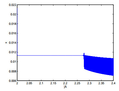
Figure 1.
Flip bifurcation diagram of map (3) in the ( \alpha , x) plane for \beta_{1} = 1, \beta_{2} = 0.5, h_{1} = 0.05, h_{2} = 0.1. The initial value is (0.0213, 0.2326).


In an earlier paper, Cruz-Uribe, Rodney and Rosta proved an equivalence between weighted Poincaré inequalities and the existence of weak solutions to a family of Neumann problems related to a degenerate p-Laplacian. Here we prove a similar equivalence between Poincaré inequalities in variable exponent spaces and solutions to a degenerate p(⋅)-Laplacian, a non-linear elliptic equation with nonstandard growth conditions.
Citation: David Cruz-Uribe, Michael Penrod, Scott Rodney. Poincaré inequalities and Neumann problems for the variable exponent setting[J]. Mathematics in Engineering, 2022, 4(5): 1-22. doi: 10.3934/mine.2022036
| [1] | Yongsheng Lei, Meng Ding, Tianliang Lu, Juhao Li, Dongyue Zhao, Fushi Chen . A novel approach for enhanced abnormal action recognition via coarse and precise detection stage. Electronic Research Archive, 2024, 32(2): 874-896. doi: 10.3934/era.2024042 |
| [2] | Ming Wei, Congxin Yang, Bo Sun, Binbin Jing . A multi-objective optimization model for green demand responsive airport shuttle scheduling with a stop location problem. Electronic Research Archive, 2023, 31(10): 6363-6383. doi: 10.3934/era.2023322 |
| [3] | Bin Zhang, Zhenyu Song, Xingping Huang, Jin Qian, Chengfei Cai . A practical object detection-based multiscale attention strategy for person reidentification. Electronic Research Archive, 2024, 32(12): 6772-6791. doi: 10.3934/era.2024317 |
| [4] | Manal Abdullah Alohali, Mashael Maashi, Raji Faqih, Hany Mahgoub, Abdullah Mohamed, Mohammed Assiri, Suhanda Drar . Spotted hyena optimizer with deep learning enabled vehicle counting and classification model for intelligent transportation systems. Electronic Research Archive, 2023, 31(7): 3704-3721. doi: 10.3934/era.2023188 |
| [5] | Eduardo Paluzo-Hidalgo, Rocio Gonzalez-Diaz, Guillermo Aguirre-Carrazana . Emotion recognition in talking-face videos using persistent entropy and neural networks. Electronic Research Archive, 2022, 30(2): 644-660. doi: 10.3934/era.2022034 |
| [6] | Mohd. Rehan Ghazi, N. S. Raghava . Securing cloud-enabled smart cities by detecting intrusion using spark-based stacking ensemble of machine learning algorithms. Electronic Research Archive, 2024, 32(2): 1268-1307. doi: 10.3934/era.2024060 |
| [7] | Ming Wei, Shaopeng Zhang, Bo Sun . Airport passenger flow, urban development and nearby airport capacity dynamic correlation: 2006-2019 time-series data analysis for Tianjin city, China. Electronic Research Archive, 2022, 30(12): 4447-4468. doi: 10.3934/era.2022226 |
| [8] | Hui Yao, Yaning Fan, Xinyue Wei, Yanhao Liu, Dandan Cao, Zhanping You . Research and optimization of YOLO-based method for automatic pavement defect detection. Electronic Research Archive, 2024, 32(3): 1708-1730. doi: 10.3934/era.2024078 |
| [9] | Ming Wei, Shaopeng Zhang, Bo Sun . Comprehensive operating efficiency measurement of 28 Chinese airports using a two-stage DEA-Tobit method. Electronic Research Archive, 2023, 31(3): 1543-1555. doi: 10.3934/era.2023078 |
| [10] | Peng Lu, Xinpeng Hao, Wenhui Li, Congqin Yi, Ru Kong, Teng Wang . ECF-YOLO: An enhanced YOLOv8 algorithm for ship detection in SAR images. Electronic Research Archive, 2025, 33(5): 3394-3409. doi: 10.3934/era.2025150 |
In an earlier paper, Cruz-Uribe, Rodney and Rosta proved an equivalence between weighted Poincaré inequalities and the existence of weak solutions to a family of Neumann problems related to a degenerate p-Laplacian. Here we prove a similar equivalence between Poincaré inequalities in variable exponent spaces and solutions to a degenerate p(⋅)-Laplacian, a non-linear elliptic equation with nonstandard growth conditions.
In biological systems, the continuous predator-prey model has been successfully investigated and many interesting results have been obtained (cf. [1,2,3,4,5,6,7,8,9] and the references therein). Moreover, based on the continuous predator-prey model, many human factors, such as time delay [10,11,12], impulsive effect [13,14,15,16,17,18,19,20], Markov Switching [21], are considered. The existing researches mainly focus on stability, periodic solution, persistence, extinction and boundedness [22,23,24,25,26,27,28].
In 2011, the authors [28] considered the system incorporating a modified version of Leslie-Gower functional response as well as that of the Holling-type Ⅲ:
| {˙x(t)=x(a1−bx−c1y2x2+k1),˙y(t)=y(a2−c2yx+k2). | (1) |
With the diffusion of the species being also taken into account, the authors [28] studied a reaction-diffusion predator-prey model, and gave the stability of this model.
In model (1) x represents a prey population, y represents a predator with population, a1 and a2 represent the growth rate of prey x and predator y respectively, constant b represents the strength of competition among individuals of prey x, c1 measures the maximum value of the per capita reduction rate of prey x due to predator y, k1 and k2 represent the extent to which environment provides protection to x and to y respectively, c2 admits a same meaning as c1. All the constants a1,a2,b,c1,c2,k1,k2 are positive parameters.
However, provided with experimental and numerical researches, it has been obtained that bifurcation is a widespread phenomenon in biological systems, from simple enzyme reactions to complex ecosystems. In general, the bifurcation may put a population at a risk of extinction and thus hinder reproduction, so the bifurcation has always been regarded as a unfavorable phenomenon in biology [29]. This bifurcation phenomenon has attracted the attention of many mathematicians, so the research on bifurcation problem is more and more abundant [30,31,32,33,34,35,36,37,38,39,40].
Although the continuous predator-prey model has been successfully applied in many ways, its disadvantages are also obvious. It requires that the species studied should have continuous and overlapping generations. In fact, we have noticed that many species do not have these characteristics, such as salmon, which have an annual spawning season and are born at the same time each year. For the population with non-overlapping generation characteristics, the discrete time model is more practical than the continuous model [38], and discrete models can generate richer and more complex dynamic properties than continuous time models [39]. In addition, since many continuous models cannot be solved by symbolic calculation, people usually use difference equations for approximation and then use numerical methods to solve the continuous model.
In view of the above discussion, the study of discrete system is paid more and more attention by mathematicians. Many latest research works have focused on flip bifurcation for different models, such as, discrete predator-prey model [41,42]; discrete reduced Lorenz system [43]; coupled thermoacoustic systems [44]; mathematical cardiac system [45]; chemostat model [46], etc.
For the above reasons, we will study from different perspectives in this paper, focusing on the discrete scheme of Eq (1).
In order to get a discrete form of Eq (1), we first let
| u=ba1x,v=c1a1y,τ=a1t, |
and rewrite u,v,τ as x,y,t, then (1) changes into:
| {˙x(t)=x(1−x−β1y2x2+h1),˙y(t)=αy(1−β2yx+h2), | (2) |
where β1=b2c1a1,h1=b2k1a21,α=a2c1,β2=c2bc1a2,h2=bk2a1.
Next, we use Euler approximation method, i.e., let
| dxdt≈xn+1−xn△t,dydt≈yn+1−yn△t, |
where △t denotes a time step, xn,yn and xn+1,yn+1 represent consecutive points. Provided with Euler approximation method with the time step △t=1, (2) changes into a two-dimensional discrete dynamical system:
| {xn+1=xn+xn(1−xn−β1y2nx2n+h1),yn+1=yn+αyn(1−β2ynxn+h2). | (3) |
For the sake of analysis, we rewrite (3) in the following map form:
| (xy)↦(x+x(1−x−β1y2x2+h1)y+αy(1−β2yx+h2)). | (4) |
In this paper, we will consider the effect of the coefficients of map (4) on the dynamic behavior of the map (4). Our goal is to show how a flipped bifurcation of map (4) can appear under some certain conditions.
The remainder of the present paper is organized as follows. In section 2, we discuss the fixed points of map (4) including existence and stability. In section 3, we investigate the flip bifurcation at equilibria E2 and E∗. It has been proved that map (4) can undergo the flip bifurcation provided with that some values of parameters be given certain. In section 4, we give an example to support the theoretical results of the present paper. As the conclusion, we make a brief discussion in section 5.
Obviously, E1(1,0) and E2(0,h2β2) are fixed points of map (4). Given the biological significance of the system, we focus on the existence of an interior fixed point E∗(x∗,y∗), where x∗>0,y∗>0 and satisfy
| 1−x∗=β1(y∗)2(x∗)2+h1,x∗+h2=β2y∗, |
i.e., x∗ is the positive root of the following cubic equation:
| β22x3+(β1−β22)x2+(β22h1+2β1h2)x+β1h22−β22h1=0. | (5) |
Based on the relationship between the roots and the coefficients of Eq (5), we have
Lemma 2.1 Assume that β1h22−β22h1<0, then Eq (5) has least one positive root, and in particular
(ⅰ) a unique positive root, if β1≥β22;
(ⅱ) three positive roots, if β1<β22.
The proof of Lemma 2.1 is easy, and so it is omitted.
In order to study the stability of equilibria, we first give the Jacobian matrix J(E) of map (4) at any a fixed point E(x,y), which can be written as
| J(E)=(2−2x−β1y2(h1−x2)(x2+h1)2−2β1xyx2+h1αβ2y2(x+h2)21+α−2αβ2yx+h2). |
For equilibria E1, we have
| J(E1)=(0001+α). |
The eigenvalues of J(E1) are λ1=0,λ2=1+α with λ2>1 due to the constant α>0, so E1(1,0) is a saddle.
For equilibria E2, note that
| J(E2)=(2−β1h22β22h10αβ21−α), |
then the eigenvalues of J(E2) are λ1=2−β1h22β22h1,λ2=1−α, and so we get
Lemma 2.2 The fixed point E2(0,h2β2) is
(ⅰ) a sink if 1<β1h22β22h1<3 and 0<α<2;
(ⅱ) a source if β1h22β22h1<1 or β1h22β22h1>3 and α>2;
(ⅲ) a a saddle if 1<β1h22β22h1<3 and α>2, or, β1h22β22h1<1 or β1h22β22h1>3 and 0<α<2;
(ⅳ) non-hyperbolic if β1h22β22h1=1 or β1h22β22h1=3 or α=2.
In this section, we will use the relevant results of literature [38,39,40] to study the flip bifurcation at equilibria E2 and E∗.
Based on (ⅲ) in Lemma 2.2, it is known that if α=2, the eigenvalues of J(E2) are: λ1=2−β1h22β22h1,λ2=−1. Define
| Fl={(β1,β2,h1,h2,α):α=2,β1,β2,h1,h2>0}. |
We conclude that a flip bifurcation at E2(0,h2β2) of map (4) can appear if the parameters vary in a small neighborhood of the set Fl.
To study the flip bifurcation, we take constant α as the bifurcation parameter, and transform E2(0,h2β2) into the origin. Let e=2−β1h22β22h1,α1=α−2, and
| u(n)=x(n),v(n)=y(n)−h2β2, |
then map (4) can be turned into
| (uv)↦(eu−u2−2β1h2β2h1uv+O((|u|+|v|+|α1|)3)2β2u−v−2β2h2u2−2β2h2v2+4h2uv+α1β2u−α1v−α1β2h2u2−α1β2h2v2+2α1h2uv+O((|u|+|v|+|α1|)3)). | (6) |
Let
| T1=(1+e02β21), |
then by the following invertible transformation:
| (uv)=T1(sw), |
map (6) turns into
| (sw)↦(es−(1+e)s2−2β1h2β2h1s(2sβ2+w)+O(|s|+|w|+|α1|)3−w+F2(s,w,α1)), | (7) |
where
| F2=2β2[(1+e)s2+2β1h2β2h1s(2sβ2+w)]−2β2h2(1+e)2s2−2β2h2(2sβ2+w)2+4(1+e)h2s(2sβ2+w) |
| +(1+e)α1β2s−α1(2sβ2+w)−(1+e)2α1β2h2s2−α1β2h2(2sβ2+w)2 |
| +2(1+e)α1h2s(2sβ2+w)+O(|s|+|w|+|α1|)3. |
Provided with the center manifold theorem (Theorem 7 in [40]), it can be obtained that there will exist a center manifold Wc(0,0) for map (7), and the center manifold Wc(0,0) can be approximated as:
| Wc(0,0)={(w,s,α1)∈R3:s=aw2+bwα1+c(α1)2+O(|w|+|α1|)3}. |
As the center manifold satisfies:
| s=a(−w+F2)2+b(−w+F2)α1+c(α1)2=e(aw2+bwα1+c(α1)2)−(1+e)(aw2+bwα1+c(α1)2)2−2β1h2β2h1(aw2+bwα1+c(α1)2)(2β2(aw2+bwα1+c(α1)2)+w)+O(|s|+|w|+|α1|)3, |
it can be obtained by comparing the coefficients of the above equality that a=0,b=0,c=0, so the center manifold of map (7) at E2(0,h2β2) is s=0. Then map (7) restricted to the center manifold turns into
| w(n+1)=−w(n)−α1w(n)−2β2h2w2(n)−α1β2h2w2(n)+O(|w(n)|+|α1|)3 |
| ≜f(w,α1). |
Obviously,
| fw(0,0)=−1,fww(0,0)=−4β2h2, |
so
| (fww(0,0))22+fwww(0,0)3≠0,fwα1(0,0)=−1≠0. |
Therefore, Theorem 4.3 in [38] guarantees that map (3) undergoes a flip bifurcation at E2(0,h2β2).
Note that
| J(E∗)=(2−2x∗−β1(y∗)2(h1−(x∗)2)((x∗)2+h1)2−2β1x∗y∗(x∗)2+h1αβ21−α), |
then the characteristic equation of Jacobian matrix J(E∗) of map (3) at E∗(x∗,y∗) is:
| λ2−(1+α0−α)λ+(1−α)α0−ηα=0, | (8) |
where
| α0=2−2x∗−β1(y∗)2(h1−(x∗)2)((x∗)2+h1)2,η=−2β1x∗y∗β2((x∗)2+h1). |
Firstly, we discuss the stability of the fixed point E∗(x∗,y∗). The stability results can be described as the the following Lemma, which can be easily proved by the relations between roots and coefficients of the characteristic Eq (8), so the proof has been omitted.
Lemma 3.1 The fixed point E∗(x∗,y∗) is
(ⅰ) a sink if one of the following conditions holds.
(ⅰ.1) 0<α0+η<1, and α0−1α0+η<α<2(1+α0)1+α0+η;
(ⅰ.2) −1<α0+η<0, and α<min
(ⅰ.3) \alpha_{0}+\eta < -1, and \frac{\alpha_{0}-1}{\alpha_{0}+\eta} > \alpha > \frac{2(1+\alpha_{0})}{1+\alpha_{0}+\eta};
(ⅱ) a source if one of the following conditions holds.
(ⅱ.1) 0 < \alpha_{0}+\eta < 1, and \alpha < \min \{\frac{\alpha_{0}-1}{\alpha_{0}+\eta}, \frac{2(1+\alpha_{0})}{1+\alpha_{0}+\eta} \};
(ⅱ.2) -1 < \alpha_{0}+\eta < 0, and \frac{\alpha_{0}-1}{\alpha_{0}+\eta} < \alpha < \frac{2(1+\alpha_{0})}{1+\alpha_{0}+\eta};
(ⅱ.3) \alpha_{0}+\eta < -1, and \alpha > \max \{\frac{\alpha_{0}-1}{\alpha_{0}+\eta}, \frac{2(1+\alpha_{0})}{1+\alpha_{0}+\eta} \};
(ⅲ) a saddle if one of the following conditions holds.
(ⅲ.1) -1 < \alpha_{0}+\eta < 1, and \alpha > \frac{2(1+\alpha_{0})}{1+\alpha_{0}+\eta};
(ⅲ.2) \alpha_{0}+\eta < -1, and \alpha < \frac{2(1+\alpha_{0})}{1+\alpha_{0}+\eta};
(ⅳ) non-hyperbolic if one of the following conditions holds.
(ⅳ.1) \alpha_{0}+\eta = 1;
(ⅳ.2) \alpha_{0}+\eta\neq -1; and \alpha = \frac{2(1+\alpha_{0})}{1+\alpha_{0}+\eta};
(ⅳ.3) \alpha_{0}+\eta\neq 0, \alpha = \frac{\alpha_{0}-1}{\alpha_{0}+\eta} and (1+\alpha_{0}-\alpha)^{2} < 4((1-\alpha)\alpha_{0}-\eta\alpha).
Then based on (ⅳ.2) of Lemma 3.1 and \alpha\neq 1+\alpha_{0}, 3+\alpha_{0}, we get that one of the eigenvalues at E^{\ast}(x^{\ast}, y^{\ast}) is -1 and the other satisfies |\lambda|\neq 1. For \alpha, \beta_{1}, \beta_{2}, h_{1}, h_{2} > 0, let us define a set:
| Fl = \{(\beta_{1}, \beta_{2}, h_{1}, h_{2}, \alpha):\alpha = \frac{2(1+\alpha_{0})}{1+\alpha_{0}+\eta}, \alpha_{0}+\eta\neq -1, \alpha\neq 1+\alpha_{0}, 3+\alpha_{0} \}. |
We assert that a flip bifurcation at E^{\ast}(x^{\ast}, y^{\ast}) of map (3) can appear if the parameters vary in a small neighborhood of the set Fl.
To discuss flip bifurcation at E^{\ast}(x^{\ast}, y^{\ast}) of map (3), we choose constant \alpha as the bifurcation parameter and adopt the central manifold and bifurcation theory [38,39,40].
Let parameters (\alpha_{1}, \beta_{1}, \beta_{2}, h_{1}, h_{2})\in Fl, and consider map (3) with (\alpha_{1}, \beta_{1}, \beta_{2}, h_{1}, h_{2}), then map (3) can be described as
| \begin{align} \begin{cases} x_{n+1} = x_{n}+x_{n}(1-x_{n}-\frac{\beta_{1}y_{n}^{2}}{x_{n}^{2}+h_{1}} ), \\ y_{n+1} = y_{n}+\alpha_{1} y_{n}(1-\frac{\beta_{2}y_{n}}{x_{n}+h_{2}} ). \end{cases} \end{align} | (9) |
Obviously, map (9) has only a unique positive fixed point E^{\ast}(x^{\ast}, y^{\ast}), and the eigenvalues are \lambda_{1} = \; -\; 1, \lambda_{2} = 2+\alpha_{0}-\alpha, where |\lambda_{2}|\neq1.
Note that (\alpha_{1}, \beta_{1}, \beta_{2}, h_{1}, h_{2})\in Fl, then \alpha_{1} = \frac{2(1+\alpha_{0})}{1+\alpha_{0}+\eta}. Let |\alpha^{\ast}| small enough, and consider the following perturbation of map (9) described by
| \begin{align} \begin{cases} x_{n+1} = x_{n}+x_{n}(1-x_{n}-\frac{\beta_{1}y_{n}^{2}}{x_{n}^{2}+h_{1}} ), \\ y_{n+1} = y_{n}+(\alpha_{1}+\alpha^{\ast}) y_{n}(1-\frac{\beta_{2}y_{n}}{x_{n}+h_{2}} ), \end{cases} \end{align} | (10) |
with \alpha^{\ast} be a perturbation parameter.
To transform E^{\ast}(x^{\ast}, y^{\ast}) into the origin, we let u = x-x^{\ast}, v = y- y^{\ast}, then map (10) changes into
| \begin{align} \left( \begin{array}{cc} {u}\\ {v} \end{array} \right) \mapsto \left( \begin{array}{cc} {a_{1}u+a_{2}v+ a_{3}u^{2}+a_{4}uv+ a_{5}v^{2}+ a_{6}u^{3}+ a_{7}u^{2}v \; \; \; \; \; \; \; \; \; \; \; \; \; } \\ { + a_{8}uv^{2} + a_{9}v^{3} +O((|u|+|v|)^{4} )\; \; \; \; \; \; \; \; \; \; \; \; \; \; \; \; \; \; \; \; \; \; \; } \\ {b_{1}u+b_{2}v+ b_{3}u^{2}+b_{4}uv+ b_{5}v^{2}+c_{1}u\alpha^{\ast}+c_{2}v\alpha^{\ast}+c_{3}u^{2}\alpha^{\ast} }\\ {+c_{4}uv\alpha^{\ast}+c_{5}v^{2}\alpha^{\ast}+ b_{6}u^{3}+ b_{7}u^{2}v+ b_{8}uv^{2} + b_{9}v^{3}\; } \\ { +O((|u|+|v|+|\alpha^{\ast}|)^{4} )\; \; \; \; \; \; \; \; \; \; \; \; \; \; \; \; \; \; \; \; \; \; \; \; \; \; \; \; \; \; \; \; \; \; \; } \end{array} \right), \end{align} | (11) |
where
a_{1} = 2-2x^{\ast}-\beta_{1}(y^{\ast})^{2}f(0)-\beta_{1}x^{\ast}(y^{\ast})^{2}f'(0); a_{2} = -2\beta_{1}x^{\ast}y^{\ast}f(0);
a_{3} = -1-\beta_{1}(y^{\ast})^{2}f'(0)-\frac{1}{2}\beta_{1}x^{\ast}(y^{\ast})^{2}f''(0); a_{4} = -2\beta_{1}y^{\ast}f(0)-2\beta_{1}x^{\ast}y^{\ast}f'(0);
a_{5} = -\beta_{1}x^{\ast}f(0); a_{6} = -\frac{1}{2}\beta_{1}(y^{\ast})^{2}f''(0)-\frac{1}{6}\beta_{1}x^{\ast}(y^{\ast})^{2}f'''(0);
a_{7} = -\beta_{1}x^{\ast}y^{\ast}f''(0)-2\beta_{1}y^{\ast}f'(0); a_{8} = -\beta_{1}f(0)-\beta_{1}x^{\ast}f'(0), \; \; \; a_{9} = 0;
f(0) = \frac{1}{(x^{\ast})^{2}+h_{1}}, f'(0) = \frac{-2x^{\ast}}{[(x^{\ast})^{2}+h_{1}]^{2}}, f''(0) = \frac{6(x^{\ast})^{2}-2h_{1}}{[(x^{\ast})^{2}+h_{1}]^{3}}, f'''(0) = \frac{ 24x^{\ast} (h_{1}-(x^{\ast})^{2})}{[(x^{\ast})^{2}+h_{1}]^{4}}.
b_{1} = \frac{\alpha_{1}\beta_{2}(y^{\ast})^{2} }{(x^{\ast}+h_{2})^{2} }; b_{2} = 1+\alpha_{1}-\frac{\alpha_{1}\beta_{2}y^{\ast} }{x^{\ast}+h_{2}}; b_{3} = -\frac{\alpha_{1}\beta_{2}(y^{\ast})^{2} }{(x^{\ast}+h_{2})^{3} }; b_{4} = \frac{2\alpha_{1}\beta_{2}y^{\ast} }{ (x^{\ast}+h_{2})^{2} };
b_{5} = -\frac{\alpha_{1}\beta_{2} }{x^{\ast}+h_{2}}; c_{1} = \frac{\beta_{2}(y^{\ast})^{2} }{(x^{\ast}+h_{2})^{2} }; c_{2} = 1-\frac{\beta_{2}y^{\ast} }{x^{\ast}+h_{2}}; c_{3} = -\frac{\beta_{2}(y^{\ast})^{2} }{(x^{\ast}+h_{2})^{3} };
c_{4} = \frac{2\beta_{2}y^{\ast} }{(x^{\ast}+h_{2})^{2} }; c_{5} = -\frac{\beta_{2} }{x^{\ast}+h_{2} }; b_{6} = \frac{\alpha_{1}\beta_{2}(y^{\ast})^{2} }{(x^{\ast}+h_{2})^{4} }; b_{7} = -\frac{2\alpha_{1}\beta_{2}y^{\ast} }{ (x^{\ast}+h_{2})^{3} };
| b_{8} = \frac{\alpha_{1}\beta_{2} }{(x^{\ast}+h_{2})^{2} }; \; \; \; \; b_{9} = 0.\; \; \; \; \; \; \; \; \; \; \; \; \; \; \; \; \; \; \; \; \; \; \; \; \; \; \; \; \; \; \; \; \; \; \; \; \; \; \; \; \; \; \; \; \; \; \; \; \; \; \; \; \; \; \; \; \; \; \; \; \; \; \; \; \; \; \; \; \; |
Now let's construct an matrix
| \begin{gather*} T_{2} = \begin{pmatrix}a_{2} & a_{2} \\-1-a_{1} & \lambda_{2}-a_{1} \end{pmatrix}. \end{gather*} |
It's obvious that the matrix T_{2} is invertible due to \lambda_{2}\neq -1, and then we use the following invertible translation
| \left( \begin{array}{cc} {u}\\ {v} \end{array} \right) = T_{2} \left( \begin{array}{cc} {s } \\ {w } \end{array} \right), |
map (11) can be described by
| \begin{align} \left( \begin{array}{cc} {s}\\ {w} \end{array} \right) \mapsto \left( \begin{array}{cc} {-s +f_{1}(s, w, \alpha^{\ast}) } \\ {\lambda_{2}w +f_{2}(s, w, \alpha^{\ast}) } \end{array} \right), \end{align} | (12) |
where
| f_{1}(s, w, \alpha^{\ast}) = \frac{(\lambda_{2}-a_{1})a_{3}-a_{2} b_{3}}{ a_{2}(\lambda_{2}+1) }u^{2} + \frac{(\lambda_{2}-a_{1})a_{4}-a_{2} b_{4}}{ a_{2}(\lambda_{2}+1) }uv +\frac{(\lambda_{2}-a_{1})a_{5}-a_{2} b_{5}}{ a_{2}(\lambda_{2}+1) }v^{2} +\frac{(\lambda_{2}-a_{1})a_{6}-a_{2} b_{6}}{ a_{2}(\lambda_{2}+1) }u^{3} \\ \; \; \; \; \; \; \; \; \; \; \; \; \; \; \; \; +\frac{(\lambda_{2}-a_{1})a_{7}-a_{2} b_{7}}{ a_{2}(\lambda_{2}+1) }u^{2}v +\frac{(\lambda_{2}-1)a_{8}-a_{2} b_{8}}{ a_{2}(\lambda_{2}+1) }uv^{2} +\frac{(\lambda_{2}-a_{1})a_{9}-a_{2} b_{9}}{ a_{2}(\lambda_{2}+1) }v^{3}- \frac{a_{2}c_{1}}{a_{2}(\lambda_{2}+1)}u\alpha^{\ast} \\ \; \; \; \; \; \; \; \; \; \; \; \; \; \; \; \; - \frac{a_{2}c_{2}}{a_{2}(\lambda_{2}+1)}v\alpha^{\ast}- \frac{a_{2}c_{3}}{a_{2}(\lambda_{2}+1)}u^{2}\alpha^{\ast} - \frac{a_{2}c_{4}}{a_{2}(\lambda_{2}+1)}uv\alpha^{\ast} - \frac{a_{2}c_{5}}{a_{2}(\lambda_{2}+1)}v^{2}\alpha^{\ast} \\ \; \; \; \; \; \; \; \; \; \; \; \; \; \; \; \; +O((|s|+ |w|+|\alpha^{\ast}| )^{4}), \\ f_{2}(s, w, \alpha^{\ast}) = \frac{(a_{1}+1)a_{3}+a_{2} b_{3}}{ a_{2}(\lambda_{2}+1) }u^{2} + \frac{(a_{1}+1)a_{4}+a_{2} b_{4}}{ a_{2}(\lambda_{2}+1) }uv +\frac{(a_{1}+1)a_{5}+a_{2} b_{5}}{ a_{2}(\lambda_{2}+1) }v^{2} +\frac{(a_{1}+1)a_{6}+a_{2} b_{6}}{ a_{2}(\lambda_{2}+1) }u^{3} \\ \; \; \; \; \; \; \; \; \; \; \; \; \; \; \; \; +\frac{(a_{1}+1)a_{7}+a_{2} b_{7}}{ a_{2}(\lambda_{2}+1) }u^{2}v +\frac{(a_{1}+1)a_{8}+a_{2} b_{8}}{ a_{2}(\lambda_{2}+1) }uv^{2}+\frac{(a_{1}+1)a_{9}+a_{2} b_{9}}{ a_{2}(\lambda_{2}+1) }v^{3}+ \frac{a_{2}c_{1}}{a_{2}(\lambda_{2}+1)}u\alpha^{\ast}\\ \; \; \; \; \; \; \; \; \; \; \; \; \; \; \; \; + \frac{a_{2}c_{2}}{a_{2}(\lambda_{2}+1)}v\alpha^{\ast}+ \frac{a_{2}c_{3}}{a_{2}(\lambda_{2}+1)}u^{2}\alpha^{\ast}+ \frac{a_{2}c_{4}}{a_{2}(\lambda_{2}+1)}uv\alpha^{\ast} + \frac{a_{2}c_{5}}{a_{2}(\lambda_{2}+1)}v^{2}\alpha^{\ast}\\ \; \; \; \; \; \; \; \; \; \; \; \; \; \; \; \; +O((|s|+ |w|+|\alpha^{\ast}| )^{4}), |
with
u = a_{2}(s+w), v = (\lambda_{2}-a_{1})w-(a_{1}+1)s;
u^{2} = (a_{2}(s+w))^{2};
uv = (a_{2}(s+w))((\lambda_{2}-a_{1})w-(a_{1}+1)s);
v^{2} = ((\lambda_{2}-a_{1})w-(a_{1}+1)s)^{2};
u^{3} = (a_{2}(s+w))^{3};
u^{2}v = (a_{2}(s+w))^{2}((\lambda_{2}-a_{1})w-(a_{1}+1)s);
uv^{2} = (a_{2}(s+w))((\lambda_{2}-a_{1})w-(a_{1}+1)s)^{2};
v^{3} = ((\lambda_{2}-a_{1})w-(a_{1}+1)s)^{3}.
In the following, we will study the center manifold of map (12) at fixed point (0, 0) in a small neighborhood of \alpha^{\ast} = 0. The well-known center manifold theorem guarantee that a center manifold W^{c}(0, 0) can exist, and it can be approximated as follows
| W^{c}(0, 0) = \{(s, w, \alpha^{\ast})\in R^{3}:w = d_{1}s^{2}+d_{2}s\alpha^{\ast}+d_{3}(\alpha^{\ast})^{2}+ O(( |s|+ |\alpha^{\ast}|)^{3}) \}, |
which satisfies
| w = d_{1}(-s+f_{1}(s, w, \alpha^{\ast}))^{2}+d_{2}(-s+f_{1}(s, w, \alpha^{\ast}))\alpha^{\ast}+d_{3}(\alpha^{\ast})^{2} |
| = \lambda_{2}( d_{1}s^{2}+d_{2}s\alpha^{\ast}+d_{3}(\alpha^{\ast})^{2} )+f_{2}(s, w, \alpha^{\ast}).\; \; \; \; \; \; \; \; \; \; \; \; \; \; \; \; \; \; |
By comparing the coefficients of the above equation, we have
| d_{1} = \frac{a_{2}((a_{1}+1)a_{3}+a_{2}b_{3})}{1-\lambda_{2}^{2}}-\frac{(a_{1}+1)((a_{1}+1)a_{4}+a_{2}b_{4})}{1-\lambda_{2}^{2}}+ \frac{(a_{1}+1)^{2}((a_{1}+1)a_{5}+a_{2}b_{5})}{1-\lambda_{2}^{2}}, \\ d_{2} = \frac{c_{2}(a_{1}+1) -a_{2}c_{1} }{(1+\lambda_{2})^{2}}, \; \; \; \; \; \; d_{3} = 0.\; \; \; \; \; \; \; \; \; \; \; \; \; \; \; \; \; \; \; \; \; \; \; \; \; \; \; \; \; \; \; \; \; \; \; \; \; \; \; \; \; \; \; \; \; \; \; \; \; \; \; \; \; \; \; \; \; \; \; \; \; \; \; \; \; \; \; \; |
So, restricted to the center manifold W^{c}(0, 0), map (12) turns into
| \begin{align} s \mapsto -s+e_{1}s^{2}+e_{2}s\alpha^{\ast}+e_{3}s^{2}\alpha^{\ast}+e_{4}s(\alpha^{\ast})^{2}+e_{5}s^{3}+O(( |s|+ |\alpha^{\ast}|)^{4}) \\ \triangleq F_{2}(s, \alpha^{\ast}), \; \; \; \; \; \; \; \; \; \; \; \; \; \; \; \; \; \; \; \; \; \; \; \; \; \; \; \; \; \; \; \; \; \; \; \; \; \; \; \; \; \; \; \; \; \; \; \; \; \; \; \; \; \; \; \; \; \; \; \; \; \; \; \; \; \; \; \; \; \end{align} | (13) |
where
e_{1} = A_{1}a_{2}^{2}-A_{2}a_{2}(a_{1}+1)+ A_{3}(a_{1}+1)^{2};
e_{2} = -A_{8}a_{2}+ A_{9}(a_{1}+1);
e_{3} = 2A_{1}d_{2}a_{2}^{2}+ A_{2}a_{2}d_{2}(\lambda_{2}-2a_{1}-1)-2A_{3}d_{2}(\lambda_{2}-a_{1})(a_{1}+1)-A_{8}a_{2}d_{1}
-A_{9}(\lambda_{2}-a_{1})d_{1}-A_{10}a_{2}^{2}+A_{11}a_{2}(a_{1}+1)-A_{12}(a_{1}+1)^{2};
e_{4} = -A_{8}a_{2}d_{2}-A_{9}(\lambda_{2}-a_{1})d_{2};
e_{5} = 2A_{1}a_{2}^{2}d_{1}+A_{2}a_{2}d_{1}(\lambda_{2}-2a_{1}-1)-2A_{3}d_{1}(\lambda_{2}-a_{1})(a_{1}+1)+A_{4}a_{2}^{3}
-A_{5}a_{2}^{2}(a_{1}+1)+A_{6}a_{2}(a_{1}+1)^{2}-A_{7}(a_{1}+1)^{3};
with
A_{1} = \frac{(\lambda_{2}-a_{1})a_{3}-a_{2} b_{3}}{ a_{2}(\lambda_{2}+1) }; \; \; A_{2} = \frac{(\lambda_{2}-a_{1})a_{4}-a_{2} b_{4}}{ a_{2}(\lambda_{2}+1) }; \; \; A_{3} = \frac{(\lambda_{2}-a_{1})a_{5}-a_{2} b_{5}}{ a_{2}(\lambda_{2}+1) }; \; \; A_{4} = \frac{(\lambda_{2}-a_{1})a_{6}-a_{2} b_{6}}{ a_{2}(\lambda_{2}+1) };
A_{5} = \frac{(\lambda_{2}-a_{1})a_{7}-a_{2} b_{7}}{ a_{2}(\lambda_{2}+1) }; \; \; A_{6} = \frac{(\lambda_{2}-1)a_{8}-a_{2} b_{8}}{ a_{2}(\lambda_{2}+1) }; \; \; A_{7} = \frac{(\lambda_{2}-a_{1})a_{9}-a_{2} b_{9}}{ a_{2}(\lambda_{2}+1) }; \; \; A_{8} = \frac{a_{2}c_{1}}{a_{2}(\lambda_{2}+1)};
A_{9} = \frac{a_{2}c_{2}}{a_{2}(\lambda_{2}+1)}; \; \; \; \; \; \; \; \; A_{10} = \frac{a_{2}c_{3}}{a_{2}(\lambda_{2}+1)}; \; \; \; \; \; \; \; \; A_{11} = \frac{a_{2}c_{4}}{a_{2}(\lambda_{2}+1)}; \; \; \; \; \; \; \; \; A_{12} = \frac{a_{2}c_{5}}{a_{2}(\lambda_{2}+1)}.
To study the flip bifurcation of map (13), we define the following two discriminatory quantities
| \mu_{1} = \left( \frac{\partial^{2}F_{2}}{\partial s\partial\alpha^{\ast}}+\frac{1}{2}\frac{\partial F_{2}}{\partial\alpha^{\ast}} \frac{\partial^{2}F_{2}}{\partial s^{2}} \right )|_{(0, 0)}, |
and
| \mu_{2} = \left(\frac{1}{6} \frac{\partial^{3}F_{2}}{\partial s^{3}}+\left(\frac{1}{2} \frac{\partial^{2}F_{2}}{\partial s^{2}}\right)^{2} \right )|_{(0, 0)} |
which can be showed in [38]. Then provided with Theorem 3.1 in [38], the following result can be given as
Theorem 3.1. Assume that \mu_{1} and \mu_{2} are not zero, then a flip bifurcation can occur at E^{\ast}(x^{\ast}, y^{\ast}) of map (3) if the parameter \alpha^{\ast} varies in a small neighborhood of origin. And that when \mu_{2} > 0 (<0), the period-2 orbit bifurcated from E^{\ast}(x^{\ast}, y^{\ast}) of map (3) is stable (unstable).
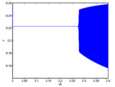
As application, we now give an example to support the theoretical results of this paper by using MATLAB. Let \beta_{1} = 1, \beta_{2} = 0.5, h_{1} = 0.05, h_{2} = 0.1, then we get from (5) that map (3) has only one positive point E^{\ast}(0.0113, 0.2226). And we further have \mu_{1} = e_{2} = 0.1134 \neq 0, \mu_{2} = e_{5}+e_{1}^{2} = -4.4869 \neq 0, which implies that all conditions of Theorem 3.1 hold, a flip bifurcation comes from E^{\ast} at the bifurcation parameter \alpha = 2.2238 , so the flip bifurcation is supercritical, i.e., the period-2 orbit is unstable.
According to Figures 1 and 2, the positive point E^{\ast}(0.0113, 0.2226) is stable for 2\leq \alpha \leq 2.4 and loses its stability at the bifurcation parameter value \alpha = 2.2238. Which implies that map (3) has complex dynamical properties.
In this paper, a predator-prey model with modified Leslie-Gower and Holling-type Ⅲ schemes is considered from another aspect. The complex behavior of the corresponding discrete time dynamic system is investigated. we have obtained that the fixed point E_{1} of map (4) is a saddle, and the fixed points E_{2} and E^{\ast} of map (4) can undergo flip bifurcation. Moreover, Theorem 3.1 tell us that the period-2 orbit bifurcated from E^{\ast}(x^{\ast}, y^{\ast}) of map (3) is stable under some sufficient conditions, which means that the predator and prey can coexist on the stable period-2 orbit. So, compared with previous studies [28] on the continuous predator-prey model, our discrete model shows more irregular and complex dynamic characteristics. The present research can be regarded as the continuation and development of the former studies in [28].
This work is supported by the National Natural Science Foundation of China (60672085), Natural Foundation of Shandong Province (ZR2016EEB07) and the Reform of Undergraduate Education in Shandong Province Research Projects (2015M139).
The authors would like to thank the referee for his/her valuable suggestions and comments which led to improvement of the manuscript.
The authors declare that they have no competing interests.
YYL carried out the proofs of main results in the manuscript. FXZ and XLZ participated in the design of the study and drafted the manuscripts. All the authors read and approved the final manuscripts.
| [1] |
M. Biegert, A priori estimates for the difference of solutions to quasi-linear elliptic equations, Manuscripta Math., 133 (2010), 273–306. doi: 10.1007/s00229-010-0367-z

|
| [2] | D. Cruz-Uribe, A. Fiorenza, Variable Lebesgue spaces, Heidelberg: Birkhäuser/Springer, 2013. |
| [3] |
D. Cruz-Uribe, K. Moen, S. Rodney, Matrix \mathcal A_p weights, degenerate Sobolev spaces, and mappings of finite distortion, J. Geom. Anal., 26 (2016), 2797–2830. doi: 10.1007/s12220-015-9649-8
|
| [4] |
D. Cruz-Uribe, S. Rodney, Bounded weak solutions to elliptic PDE with data in Orlicz spaces, J. Differ. Equations, 297 (2021), 409–432. doi: 10.1016/j.jde.2021.06.025
|
| [5] |
D. Cruz-Uribe, S. Rodney, E. Rosta, Poincaré inequalities and neumann problems for the p-laplacian, Can. Math. Bull., 61 (2018), 738–753. doi: 10.4153/CMB-2018-001-6
|
| [6] | L. Diening, P. Harjulehto, P. Hästö, M. Růžička, Lebesgue and Sobolev spaces with variable exponents, Heidelberg: Springer, 2011. |
| [7] | D. E. Edmunds, J. Lang, O. Méndez, Differential operators on spaces of variable integrability, Hackensack, NJ: World Scientific Publishing Co. Pte. Ltd., 2014. |
| [8] |
E. B. Fabes, C. E. Kenig, R. P. Serapioni, The local regularity of solutions of degenerate elliptic equations, Commun. Part. Diff. Eq., 7 (1982), 77–116. doi: 10.1080/03605308208820218
|
| [9] |
P. Harjulehto, P. Hästö, Út V. Lê, M. Nuortio, Overview of differential equations with non-standard growth, Nonlinear Anal., 72 (2010), 4551–4574. doi: 10.1016/j.na.2010.02.033
|
| [10] |
K. Ho, I. Sim, Existence results for degenerate p(x)-Laplace equations with Leray-Lions type operators, Sci. China Math., 60 (2017), 133–146. doi: 10.1007/s11425-015-0385-0
|
| [11] |
Y. H. Kim, L. Wang, C. Zhang, Global bifurcation for a class of degenerate elliptic equations with variable exponents, J. Math. Anal. Appl., 371 (2010), 624–637. doi: 10.1016/j.jmaa.2010.05.058
|
| [12] |
L. Kong, A degenerate elliptic system with variable exponents, Sci. China Math., 62 (2019), 1373–1390. doi: 10.1007/s11425-018-9409-5
|
| [13] | P. Lindqvist, Notes on the p-laplace equation, 2006, preprint. |
| [14] |
G. Mingione, Regularity of minima: an invitation to the dark side of the calculus of variations, Appl. Math., 51 (2006), 355–426. doi: 10.1007/s10778-006-0110-3
|
| [15] |
A. Ron, Z. Shen, Frames and stable bases for shift-invariant subspaces of L_2(\mathbf R^d), Can. J. Math., 47 (1995), 1051–1094. doi: 10.4153/CJM-1995-056-1
|
| [16] | V. D. Rǎdulescu, D. D. Repovš, Partial differential equations with variable exponents, Boca Raton, FL: CRC Press, 2015. |
| [17] | E. T. Sawyer, R. L. Wheeden, Hölder continuity of weak solutions to subelliptic equations with rough coefficients, Mem. Amer. Math. Soc., 180 (2006), 847. |
| [18] | E. T. Sawyer, R. L. Wheeden, Degenerate Sobolev spaces and regularity of subelliptic equations, T. Am. Math. Soc., 362 (2010), 1869–1906. |
| [19] | R. E. Showalter, Monotone operators in Banach spaces and nonlinear partial differential equations, Providence, RI: American Mathematical Society, 1997. |
| 1. | Daoyong Fu, Rui Mou, Ke Yang, Wei Li, Songchen Han, Active Vision-Based Alarm System for Overrun Events of Takeoff and Landing Aircraft, 2025, 25, 1530-437X, 5745, 10.1109/JSEN.2024.3514703 |
David Cruz-Uribe, Michael Penrod, Scott Rodney. Poincaré inequalities and Neumann problems for the variable exponent setting[J]. Mathematics in Engineering, 2022, 4(5): 1-22. doi: 10.3934/mine.2022036

 DownLoad:

