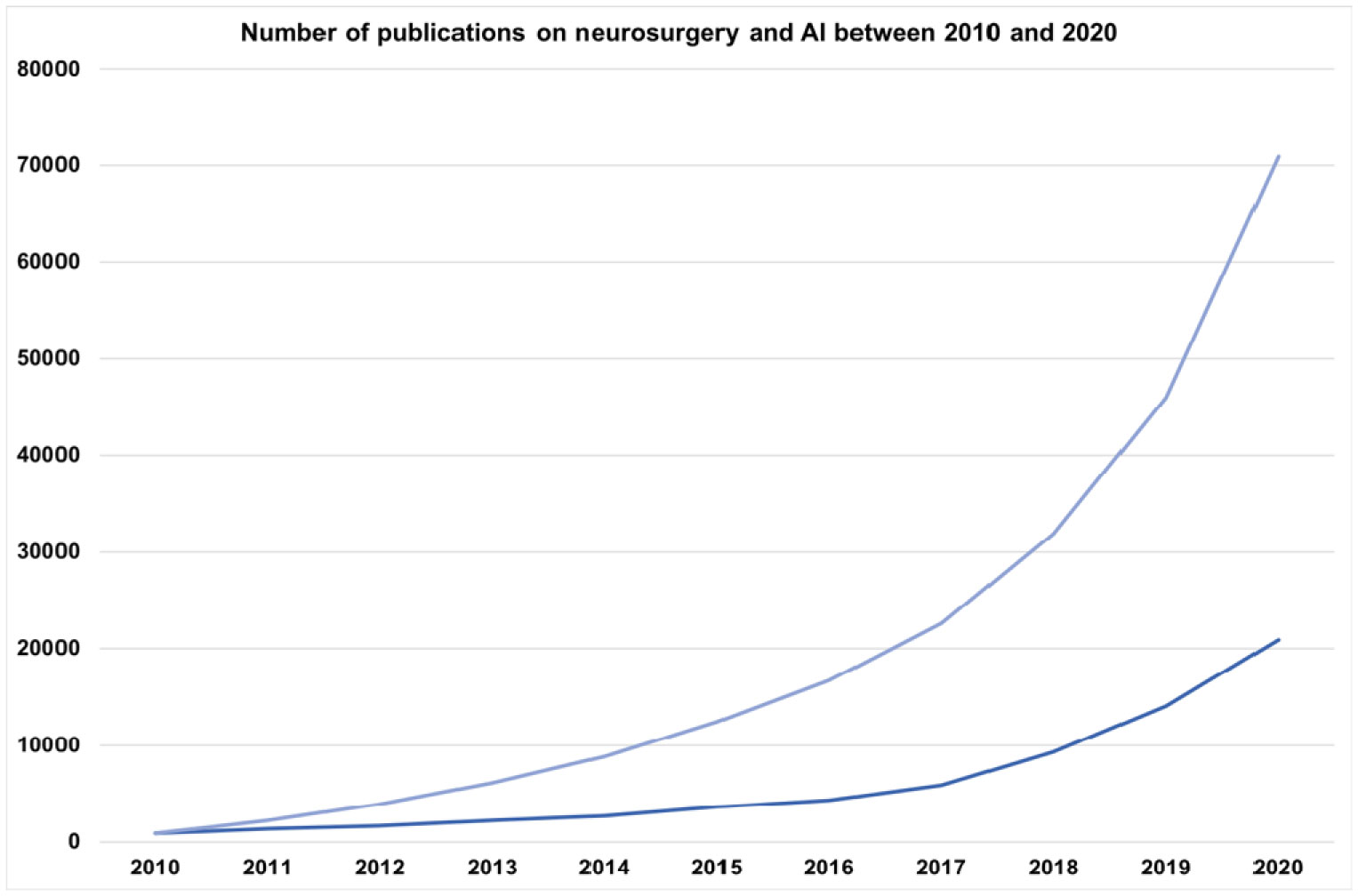
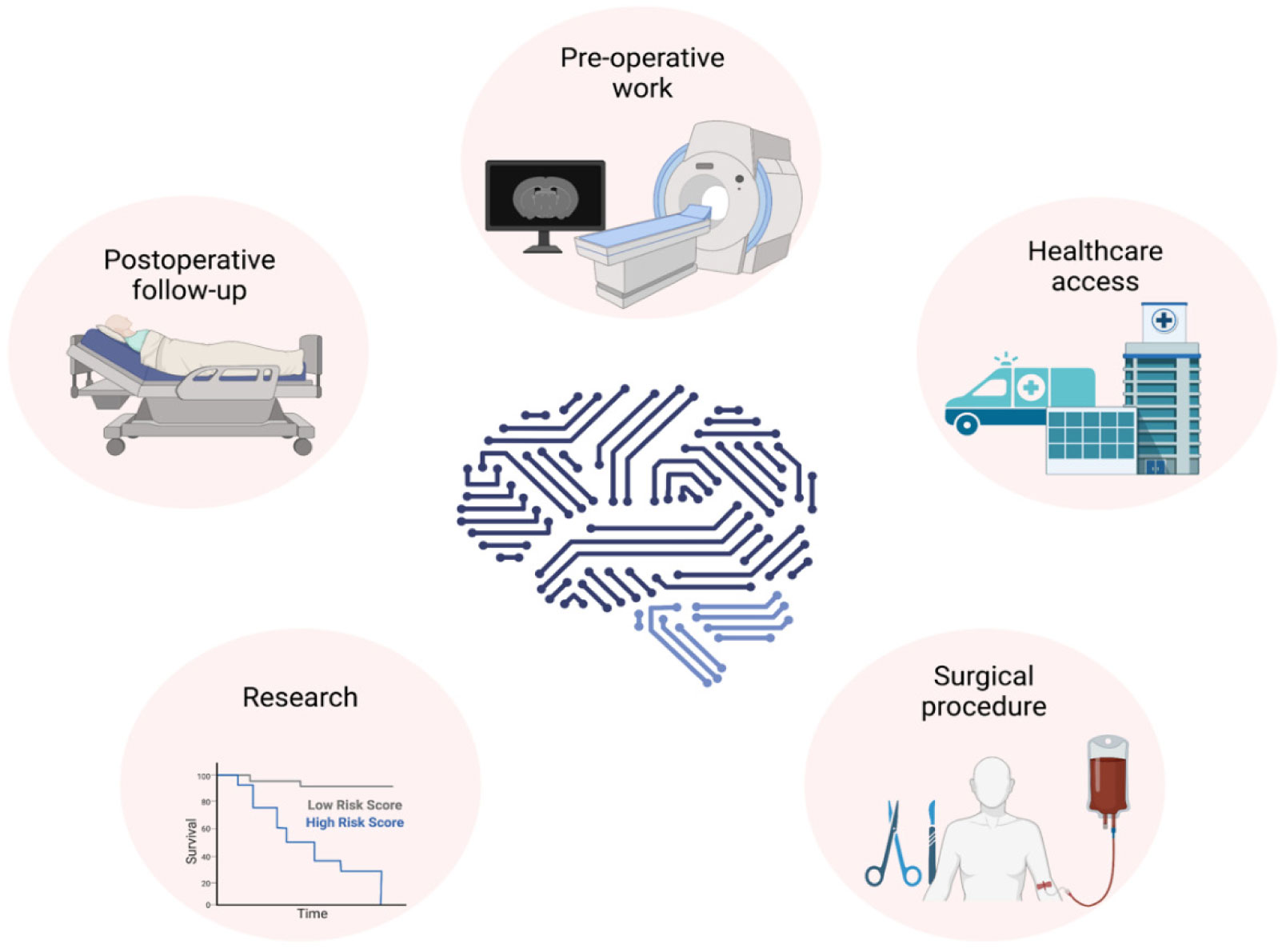
Neurosurgeons receive extensive and lengthy training to equip themselves with various technical skills, and neurosurgery require a great deal of pre-, intra- and postoperative clinical data collection, decision making, care and recovery. The last decade has seen a significant increase in the importance of artificial intelligence (AI) in neurosurgery. AI can provide a great promise in neurosurgery by complementing neurosurgeons' skills to provide the best possible interventional and noninterventional care for patients by enhancing diagnostic and prognostic outcomes in clinical treatment and help neurosurgeons with decision making during surgical interventions to improve patient outcomes. Furthermore, AI is playing a pivotal role in the production, processing and storage of clinical and experimental data. AI usage in neurosurgery can also reduce the costs associated with surgical care and provide high-quality healthcare to a broader population. Additionally, AI and neurosurgery can build a symbiotic relationship where AI helps to push the boundaries of neurosurgery, and neurosurgery can help AI to develop better and more robust algorithms. This review explores the role of AI in interventional and noninterventional aspects of neurosurgery during pre-, intra- and postoperative care, such as diagnosis, clinical decision making, surgical operation, prognosis, data acquisition, and research within the neurosurgical arena.
Citation: Mohammad Mofatteh. Neurosurgery and artificial intelligence[J]. AIMS Neuroscience, 2021, 8(4): 477-495. doi: 10.3934/Neuroscience.2021025
Neurosurgeons receive extensive and lengthy training to equip themselves with various technical skills, and neurosurgery require a great deal of pre-, intra- and postoperative clinical data collection, decision making, care and recovery. The last decade has seen a significant increase in the importance of artificial intelligence (AI) in neurosurgery. AI can provide a great promise in neurosurgery by complementing neurosurgeons' skills to provide the best possible interventional and noninterventional care for patients by enhancing diagnostic and prognostic outcomes in clinical treatment and help neurosurgeons with decision making during surgical interventions to improve patient outcomes. Furthermore, AI is playing a pivotal role in the production, processing and storage of clinical and experimental data. AI usage in neurosurgery can also reduce the costs associated with surgical care and provide high-quality healthcare to a broader population. Additionally, AI and neurosurgery can build a symbiotic relationship where AI helps to push the boundaries of neurosurgery, and neurosurgery can help AI to develop better and more robust algorithms. This review explores the role of AI in interventional and noninterventional aspects of neurosurgery during pre-, intra- and postoperative care, such as diagnosis, clinical decision making, surgical operation, prognosis, data acquisition, and research within the neurosurgical arena.
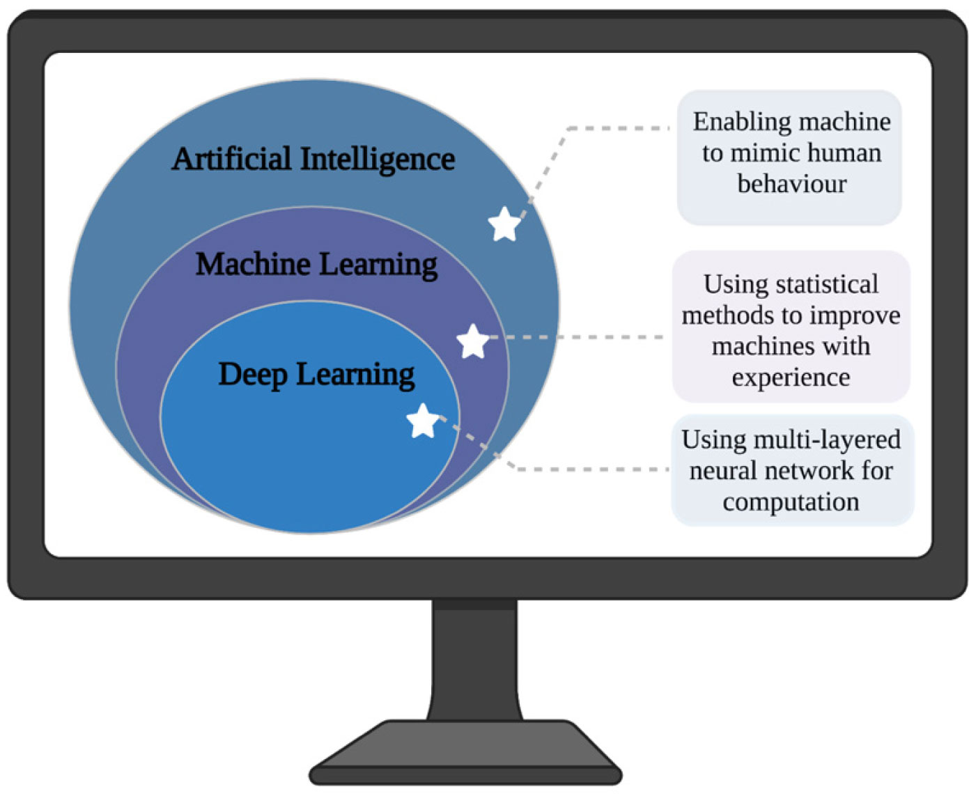
artificial intelligence
brain-computer interface
computer-assisted diagnosis
computerised tomography
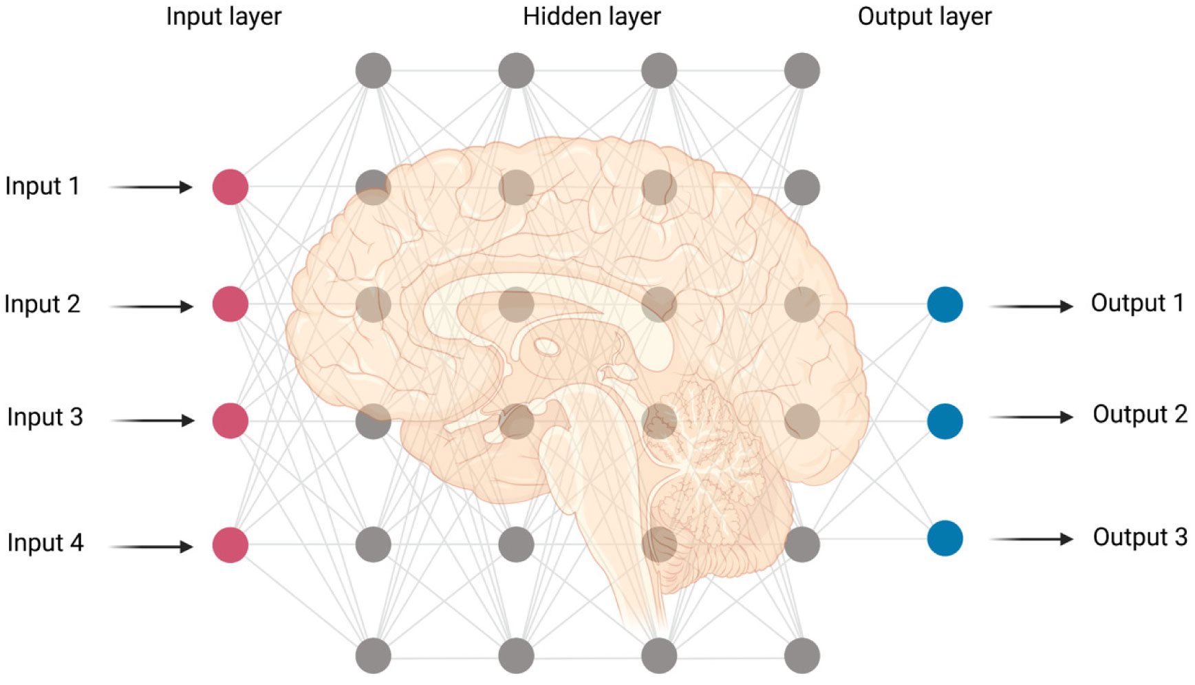
deep learning
machine learning
magnetic resonance imaging
traumatic brain injury
temporal lobe epilepsy

| [1] |
Wise J (2020) Life as a neurosurgeon. BMJ 368: m395. doi: 10.1136/bmj.m395

|
| [2] |
Kaptigau WM, Rosenfeld JV, Kevau I, et al. (2016) The establishment and development of neurosurgery services in Papua New Guinea. World J Surg 40: 251-257. doi: 10.1007/s00268-015-3268-1
|
| [3] |
Rolston JD, Zygourakis CC, Han SJ, et al. (2014) Medical errors in neurosurgery. Surg Neurol Int 5: S435-S440. doi: 10.4103/2152-7806.142777
|
| [4] |
Kwoh YS, Hou J, Jonckheere EA, et al. (1988) A robot with improved absolute positioning accuracy for CT guided stereotactic brain surgery. IEEE Trans Biomed Eng 35: 153-160. doi: 10.1109/10.1354
|
| [5] | Aziz T, Roy H (2021) Deep Brain Stimulation. Oxford Research Encyclopedia of Psychology Oxford University Press. |
| [6] |
Panesar SS, Kliot M, Parrish R, et al. (2020) Promises and perils of artificial intelligence in neurosurgery. Neurosurgery 87: 33-44. doi: 10.1093/neuros/nyz471
|
| [7] | Bohl MA, Oppenlander ME, Spetzler R (2016) A prospective cohort evaluation of a robotic, auto-navigating operating microscope. Cureus 8: e662-e662. |
| [8] |
Lanfranco AR, Castellanos AE, Desai JP, et al. (2004) Robotic surgery: a current perspective. Ann Surg 239: 14-21. doi: 10.1097/01.sla.0000103020.19595.7d
|
| [9] |
Shimizu S, Kuroda H, Mochizuki T, et al. (2020) Ergonomics-based positioning of the operating handle of surgical microscopes. Neurol Med-Chir 60: 313-316. doi: 10.2176/nmc.rc.2020-0018
|
| [10] | Van Bavel J (2013) The world population explosion: causes, backgrounds and pro-jections for the future. Facts Views Vision Obgyn 5: 281-291. |
| [11] |
Vaupel JW (2010) Biodemography of human ageing. Nature 464: 536-542. doi: 10.1038/nature08984
|
| [12] |
You D, Hug L, Ejdemyr S, et al. (2015) Global, regional, and national levels and trends in under-5 mortality between 1990 and 2015, with scenario-based projections to 2030: a systematic analysis by the UN Inter-agency Group for Child Mortality Estimation. Lancet 386: 2275-2286. doi: 10.1016/S0140-6736(15)00120-8
|
| [13] |
Aluttis C, Bishaw T, Frank MW (2014) The workforce for health in a globalized context-global shortages and international migration. Global Health Action 7: 23611-23611. doi: 10.3402/gha.v7.23611
|
| [14] |
Senders JT, Arnaout O, Karhade AV, et al. (2018) Natural and artificial intelligence in neurosurgery: a systematic review. Neurosurgery 83: 181-192. doi: 10.1093/neuros/nyx384
|
| [15] |
Sullivan R, Alatise OI, Anderson BO, et al. (2015) Global cancer surgery: delivering safe, affordable, and timely cancer surgery. Lancet Oncol 16: 1193-1224. doi: 10.1016/S1470-2045(15)00223-5
|
| [16] |
Michael CD, Abbas R, Graham F, et al. (2019) Global neurosurgery: the current capacity and deficit in the provision of essential neurosurgical care. Executive summary of the global neurosurgery initiative at the program in global surgery and social change. J Neurosurg 130: 1055-1064. doi: 10.3171/2017.11.JNS171500
|
| [17] |
Swagoto M, Maria P, Abbas R, et al. (2019) The global neurosurgical workforce: a mixed-methods assessment of density and growth. J Neurosurg 130: 1142-1148. doi: 10.3171/2018.10.JNS171723
|
| [18] |
Kato Y, Liew BS, Sufianov AA, et al. (2020) Review of global neurosurgery education: horizon of neurosurgery in the developing countries. Chin Neurosurg J 6: 19. doi: 10.1186/s41016-020-00194-1
|
| [19] |
Solomou G, Murphy S, Bandyopadhyay S, et al. (2020) Neurosurgery specialty training in the UK: What you need to know to be shortlisted for an interview. Ann Med Surg 57: 287-290. doi: 10.1016/j.amsu.2020.07.047
|
| [20] |
Mooney MA, Yoon S, Cole T, et al. (2019) Cost transparency in neurosurgery: a single-institution analysis of patient out-of-pocket spending in 13673 consecutive neurosurgery cases. Neurosurgery 84: 1280-1289. doi: 10.1093/neuros/nyy185
|
| [21] |
Yoon JS, Tang OY, Lawton MT (2019) Volume–cost relationship in neurosurgery: analysis of 12,129,029 admissions from the national inpatient sample. World Neurosurg 129: e791-e802. doi: 10.1016/j.wneu.2019.06.034
|
| [22] |
Obermeyer Z, Emanuel EJ (2016) Predicting the future–Big data, Machine learning, and Clinical medicine. N Engl J Med 375: 1216-1219. doi: 10.1056/NEJMp1606181
|
| [23] | Cruz JA, Wishart DS (2007) Applications of machine learning in cancer prediction and prognosis. Cancer Inform 2: 59-77. |
| [24] |
Marcus HJ, Williams S, Hughes-Hallett A, et al. (2017) Predicting surgical outcome in patients with glioblastoma multiforme using pre-operative magnetic resonance imaging: development and preliminary validation of a grading system. Neurosurg Rev 40: 621-631. doi: 10.1007/s10143-017-0817-0
|
| [25] |
Rudie JD, Rauschecker AM, Bryan RN, et al. (2019) Emerging applications of artificial intelligence in neuro-oncology. Radiology 290: 607-618. doi: 10.1148/radiol.2018181928
|
| [26] |
Deo RC (2015) Machine learning in medicine. Circulation 132: 1920-1930. doi: 10.1161/CIRCULATIONAHA.115.001593
|
| [27] |
Lane T (2018) A short history of robotic surgery. Ann R Coll Surge Engl 100: 5-7. doi: 10.1308/rcsann.supp1.5
|
| [28] |
Sheetz KH, Claflin J, Dimick JB (2020) Trends in the adoption of robotic surgery for common surgical procedures. JAMA Network Open 3: e1918911-e1918911. doi: 10.1001/jamanetworkopen.2019.18911
|
| [29] |
Topol EJ (2019) High-performance medicine: the convergence of human and artificial intelligence. Nat Med 25: 44-56. doi: 10.1038/s41591-018-0300-7
|
| [30] |
Jordan MI, Mitchell TM (2015) Machine learning: Trends, perspectives, and prospects. Science 349: 255. doi: 10.1126/science.aaa8415
|
| [31] |
Senders JT, Staples PC, Karhade AV, et al. (2018) Machine learning and neurosurgical outcome prediction: a systematic review. World Neurosurg 109: 476-486. doi: 10.1016/j.wneu.2017.09.149
|
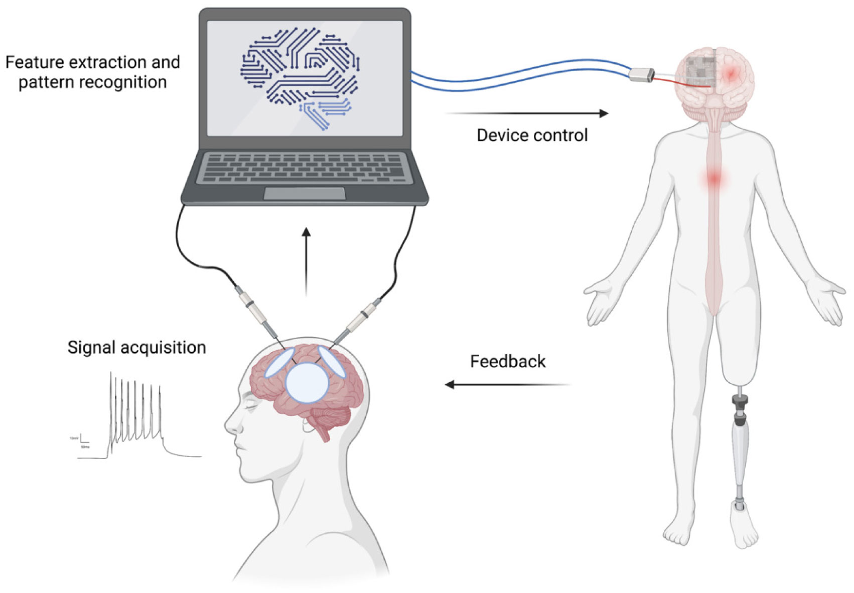
| [32] |
LeCun Y, Bengio Y, Hinton G (2015) Deep learning. Nature 521: 436-444. doi: 10.1038/nature14539
|
| [33] |
Alvin MD, Lubelski D, Alam R, et al. (2018) Spine surgeon treatment variability: the impact on costs. Global Spine J 8: 498-506. doi: 10.1177/2192568217739610
|
| [34] |
Daniels AH, Ames CP, Smith JS, et al. (2014) Variability in spine surgery procedures performed during orthopaedic and neurological surgery residency training: an analysis of ACGME case log data. J Bone Joint Surg Am 96: e196. doi: 10.2106/JBJS.M.01562
|
| [35] |
Deyo RA, Mirza SK (2006) Trends and variations in the use of spine surgery. Clin Orthop Relat Res 443: 139-146. doi: 10.1097/01.blo.0000198726.62514.75
|
| [36] |
Mroz TE, Lubelski D, Williams SK, et al. (2014) Differences in the surgical treatment of recurrent lumbar disc herniation among spine surgeons in the United States. Spine J 14: 2334-2343. doi: 10.1016/j.spinee.2014.01.037
|
| [37] |
Rasouli JJ, Shao J, Neifert S, et al. (2020) Artificial intelligence and robotics in spine surgery. Global Spine J 11: 556-564. doi: 10.1177/2192568220915718
|
| [38] |
Arvind V, Kim JS, Oermann EK, et al. (2018) Predicting surgical complications in adult patients undergoing anterior cervical discectomy and fusion using nachine learning. Neurospine 15: 329-337. doi: 10.14245/ns.1836248.124
|
| [39] |
Galbusera F, Casaroli G, Bassani T (2019) Artificial intelligence and machine learning in spine research. JOR Spine 2: e1044. doi: 10.1002/jsp2.1044
|
| [40] |
Kim JS, Merrill RK, Arvind V, et al. (2018) Examining the ability of artificial neural networks machine learning models to accurately predict complications following posterior lumbar spine fusion. Spine 43: 853-860. doi: 10.1097/BRS.0000000000002442
|
| [41] |
Emblem KE, Nedregaard B, Hald JK, et al. (2009) Automatic glioma characterization from dynamic susceptibility contrast imaging: brain tumor segmentation using knowledge-based fuzzy clustering. J Magne Reson Imaging 30: 1-10. doi: 10.1002/jmri.21815
|
| [42] |
Emblem KE, Pinho MC, Zöllner FG, et al. (2014) A generic support vector machine model for preoperative glioma survival associations. Radiology 275: 228-234. doi: 10.1148/radiol.14140770
|
| [43] |
Brady AP (2017) Error and discrepancy in radiology: inevitable or avoidable? Insights Imaging 8: 171-182. doi: 10.1007/s13244-016-0534-1
|
| [44] |
Siarkowski M, Lin K, Li SS, et al. (2020) Meta-analysis of interventions to reduce door to needle times in acute ischaemic stroke patients. BMJ Open Qual 9: e000915. doi: 10.1136/bmjoq-2020-000915
|
| [45] |
Mun SK, Wong KH, Lo S-CB, et al. (2021) Artificial Intelligence for the Future Radiology Diagnostic Service. Front Mol Biosci 7: 614258. doi: 10.3389/fmolb.2020.614258
|
| [46] |
Furlan Anthony J (2006) Time is brain. Stroke 37: 2863-2864. doi: 10.1161/01.STR.0000251852.07152.63
|
| [47] |
Fonarow Gregg C, Smith Eric E, Saver Jeffrey L, et al. (2011) Improving door-to-needle times in acute ischemic stroke. Stroke 42: 2983-2989. doi: 10.1161/STROKEAHA.111.621342
|
| [48] |
Man S, Xian Y, Holmes DN, et al. (2020) Association between thrombolytic door-to-needle time and 1-year mortality and readmission in patients with acute ischemic stroke. JAMA 323: 2170-2184. doi: 10.1001/jama.2020.5697
|
| [49] |
Nagaratnam K, Harston G, Flossmann E, et al. (2020) Innovative use of artificial intelligence and digital communication in acute stroke pathway in response to COVID-19. Future Healthcare J 7: 169-173. doi: 10.7861/fhj.2020-0034
|
| [50] |
Yamashita K, Yoshiura T, Arimura H, et al. (2008) Performance evaluation of radiologists with artificial neural network for differential diagnosis of intra-axial cerebral tumors on MR images. Am J Neuroradiol 29: 1153-1158. doi: 10.3174/ajnr.A1037
|
| [51] |
Kassahun Y, Perrone R, De Momi E, et al. (2014) Automatic classification of epilepsy types using ontology-based and genetics-based machine learning. Artif Intell Med 61: 79-88. doi: 10.1016/j.artmed.2014.03.001
|
| [52] |
Bidiwala S, Pittman T (2004) Neural network classification of pediatric posterior fossa tumors using clinical and imaging data. Pediatr Neurosurg 40: 8-15. doi: 10.1159/000076571
|
| [53] |
Zhang B, Chang K, Ramkissoon S, et al. (2017) Multimodal MRI features predict isocitrate dehydrogenase genotype in high-grade gliomas. Neuro Oncol 19: 109-117. doi: 10.1093/neuonc/now121
|
| [54] |
Titano JJ, Badgeley M, Schefflein J, et al. (2018) Automated deep-neural-network surveillance of cranial images for acute neurologic events. Nat Med 24: 1337-1341. doi: 10.1038/s41591-018-0147-y
|
| [55] |
Ueda D, Yamamoto A, Nishimori M, et al. (2018) Deep Learning for MR Angiography: Automated Detection of Cerebral Aneurysms. Radiology 290: 187-194. doi: 10.1148/radiol.2018180901
|
| [56] |
Dolz J, Betrouni N, Quidet M, et al. (2016) Stacking denoising auto-encoders in a deep network to segment the brainstem on MRI in brain cancer patients: A clinical study. Comput Med Imag Grap 52: 8-18. doi: 10.1016/j.compmedimag.2016.03.003
|
| [57] |
Cohen KB, Glass B, Greiner HM, et al. (2016) Methodological issues in predicting pediatric epilepsy surgery candidates through natural language processing and machine learning. Biomed Inform Insights 8: 11-18. doi: 10.4137/BII.S38308
|
| [58] |
Dumont TM, Rughani AI, Tranmer BI (2011) Prediction of symptomatic cerebral vasospasm after aneurysmal subarachnoid hemorrhage with an artificial neural network: feasibility and comparison with logistic regression models. World Neurosurgery 75: 57-63. doi: 10.1016/j.wneu.2010.07.007
|
| [59] |
Nielsen A, Hansen Mikkel B, Tietze A, et al. (2018) Prediction of tissue outcome and assessment of treatment effect in acute ischemic stroke using deep learning. Stroke 49: 1394-1401. doi: 10.1161/STROKEAHA.117.019740
|
| [60] |
Lüders H, Acharya J, Baumgartner C, et al. (1998) Semiological seizure classification. Epilepsia 39: 1006-1013. doi: 10.1111/j.1528-1157.1998.tb01452.x
|
| [61] |
Emblem KE, Nedregaard B, Nome T, et al. (2008) Glioma grading by using histogram analysis of blood volume heterogeneity from MR-derived cerebral blood volume maps. Radiology 247: 808-817. doi: 10.1148/radiol.2473070571
|
| [62] | Lev MH, Ozsunar Y, Henson JW, et al. (2004) Glial tumor grading and outcome prediction using dynamic spin-echo MR susceptibility mapping compared with conventional contrast-enhanced MR: confounding effect of elevated rCBV of oligodendroglimoas. Am J Neuroradiol 25: 214-221. |
| [63] |
Marcus AP, Marcus HJ, Camp SJ, et al. (2020) Improved prediction of surgical resectability in patients with glioblastoma using an artificial neural network. Sci Rep 10: 5143. doi: 10.1038/s41598-020-62160-2
|
| [64] |
Young R, Babb J, Law M, et al. (2007) Comparison of region-of-interest analysis with three different histogram analysis methods in the determination of perfusion metrics in patients with brain gliomas. J Magn Reson Imaging 26: 1053-1063. doi: 10.1002/jmri.21064
|
| [65] |
Duffau H, Capelle L (2004) Preferential brain locations of low-grade gliomas. Cancer 100: 2622-2626. doi: 10.1002/cncr.20297
|
| [66] |
Clarke LP, Velthuizen RP, Clark M, et al. (1998) MRI measurement of brain tumor response: comparison of visual metric and automatic segmentation. Magn Reson Imaging 16: 271-279. doi: 10.1016/S0730-725X(97)00302-0
|
| [67] |
Pfirrmann CWA, Metzdorf A, Zanetti M, et al. (2001) Magnetic resonance classification of lumbar intervertebral disc degeneration. Spine 26: 1873-1878. doi: 10.1097/00007632-200109010-00011
|
| [68] |
Toyoda H, Takahashi S, Hoshino M, et al. (2017) Characterizing the course of back pain after osteoporotic vertebral fracture: a hierarchical cluster analysis of a prospective cohort study. Arch Osteoporos 12: 82. doi: 10.1007/s11657-017-0377-5
|
| [69] |
Jeffrey EA, Craig M, Zhiyue JW, et al. (1997) Prediction of posterior fossa tumor type in children by means of magnetic resonance image properties, spectroscopy, and neural networks. J Neurosurg 86: 755-761. doi: 10.3171/jns.1997.86.5.0755
|
| [70] |
Kitajima M, Hirai T, Katsuragawa S, et al. (2009) Differentiation of common large sellar-suprasellar masses: effect of artificial neural network on radiologists' diagnosis performance. Acad Radiol 16: 313-320. doi: 10.1016/j.acra.2008.09.015
|
| [71] |
Christy PS, Tervonen O, Scheithauer BW, et al. (1995) Use of a neural network and a multiple regression model to predict histologic grade of astrocytoma from MRI appearances. Neuroradiology 37: 89-93. doi: 10.1007/BF00588619
|
| [72] |
Juntu J, Sijbers J, De Backer S, et al. (2010) Machine learning study of several classifiers trained with texture analysis features to differentiate benign from malignant soft-tissue tumors in T1-MRI images. J Magn Reson Imaging 31: 680-689. doi: 10.1002/jmri.22095
|
| [73] |
Zhao Z-X, Lan K, Xiao JH, et al. (2010) A new method to classify pathologic grades of astrocytomas based on magnetic resonance imaging appearances. Neurology India 58: 685-690. doi: 10.4103/0028-3886.72161
|
| [74] |
Sinha M, Kennedy CS, Ramundo, et al. (2001) Artificial neural network predicts CT scan abnormalities in pediatric patients with closed head injury. J Trauma 50: 308-312. doi: 10.1097/00005373-200102000-00018
|
| [75] |
Chiang S, Levin HS, Haneef Z (2015) Computer-automated focus lateralization of temporal lobe epilepsy using fMRI. J Magn Reson Imaging 41: 1689-1694. doi: 10.1002/jmri.24696
|
| [76] |
Berg AT, Vickrey BG, Langfitt JT, et al. (2003) The multicenter study of epilepsy surgery: recruitment and selection for surgery. Epilepsia 44: 1425-1433. doi: 10.1046/j.1528-1157.2003.24203.x
|
| [77] |
Tankus A, Yeshurun Y, Fried I (2009) An automatic measure for classifying clusters of suspected spikes into single cells versus multiunits. J Neural Eng 6: 056001. doi: 10.1088/1741-2560/6/5/056001
|
| [78] |
Anand IR, Travis MD, Zhenyu L, et al. (2010) Use of an artificial neural network to predict head injury outcome. J Neurosurg 113: 585-590. doi: 10.3171/2009.11.JNS09857
|
| [79] |
Chang K, Bai HX, Zhou H, et al. (2018) Residual convolutional neural network for the determination of IDH status in low- and high-grade gliomas from MR Imaging. Clin Cancer Res 24: 1073-1081. doi: 10.1158/1078-0432.CCR-17-2236
|
| [80] |
Yu J, Shi Z, Lian Y, et al. (2017) Noninvasive IDH1 mutation estimation based on a quantitative radiomics approach for grade II glioma. Eur Radiol 27: 3509-3522. doi: 10.1007/s00330-016-4653-3
|
| [81] |
Hollon TC, Pandian B, Adapa AR, et al. (2020) Near real-time intraoperative brain tumor diagnosis using stimulated raman histology and deep neural networks. Nat Med 26: 52-58. doi: 10.1038/s41591-019-0715-9
|
| [82] |
Gal AA, Cagle PT (2005) The 100-year anniversary of the description of the frozen section procedure. JAMA 294: 3135-3137. doi: 10.1001/jama.294.24.3135
|
| [83] | Novis D, Zarbo R (1997) Interinstitutional comparison of frozen section turnaround time. A college of American Pathologists Q-Probes study of 32868 frozen sections in 700 hospitals. Arch Pathol Lab Med 121: 559-567. |
| [84] |
Mosa ASM, Yoo I, Sheets L (2012) A systematic review of healthcare applications for smartphones. BMC Med Inform Decis Mak 12: 67. doi: 10.1186/1472-6947-12-67
|
| [85] | Bardram JE, Bossen C (2005) Mobility Work: The spatial dimension of collaboration at a hospital. CSCW 14: 131-160. |
| [86] |
Hector EJ (2016) Pediatric neurosurgery telemedicine clinics: a model to provide care to geographically underserved areas of the United States and its territories. J Neurosurg Pediatr 18: 753-757. doi: 10.3171/2016.6.PEDS16202
|
| [87] |
Reider-Demer M, Raja P, Martin N, et al. (2018) Prospective and retrospective study of videoconference telemedicine follow-up after elective neurosurgery: results of a pilot program. Neurosurg Rev 41: 497-501. doi: 10.1007/s10143-017-0878-0
|
| [88] | Susan RS (2018) Editorial. Telemedicine for elective neurosurgical routine follow-up care: a promising patient-centered and cost-effective alternative to in-person clinic visits. Neurosurg Focus 44: E18. |
| [89] |
Semple JL, Armstrong KA (2017) Mobile applications for postoperative monitoring after discharge. CMAJ 189: E22-E24. doi: 10.1503/cmaj.160195
|
| [90] |
Layard Horsfall H, Palmisciano P, Khan DZ, et al. (2021) Attitudes of the surgical team toward artificial intelligence in neurosurgery: international 2-stage cross-sectional survey. World Neurosurg 146: e724-e730. doi: 10.1016/j.wneu.2020.10.171
|
| [91] |
Tsermoulas G, Zisakis A, Flint G, et al. (2020) Challenges to neurosurgery during the coronavirus disease 2019 (COVID-19) pandemic. World Neurosurg 139: 519-525. doi: 10.1016/j.wneu.2020.05.108
|
| [92] |
Zemmar A, Lozano AM, Nelson BJ (2020) The rise of robots in surgical environments during COVID-19. Nat Mach Intell 2: 566-572. doi: 10.1038/s42256-020-00238-2
|
| [93] | Michael CD, Ronnie EB, Abbas R, et al. (2018) Pediatric neurosurgical workforce, access to care, equipment and training needs worldwide. Neurosurg Focus 45: E13. |
| [94] |
Mofatteh M (2021) Risk factors associated with stress, anxiety, and depression among university undergraduate students. AIMS Public Health 8: 36-65. doi: 10.3934/publichealth.2021004
|
| [95] |
Stein SC (2018) Cost-effectiveness research in neurosurgery: we can and we must. Neurosurgery 83: 871-878. doi: 10.1093/neuros/nyx583
|
| [96] |
Sejnowski TJ (2020) The unreasonable effectiveness of deep learning in artificial intelligence. Proc Natl Acad Sci 117: 30033-30038. doi: 10.1073/pnas.1907373117
|
| [97] |
Bell C, Shenoy P, Chalodhorn R, et al. (2008) Control of a humanoid robot by a noninvasive brain-computer interface in humans. J Neural Eng 5: 214-220. doi: 10.1088/1741-2560/5/2/012
|
| [98] |
Zhang X, Ma Z, Zheng H, et al. (2020) The combination of brain-computer interfaces and artificial intelligence: applications and challenges. Ann Transl Med 8: 712. doi: 10.21037/atm.2019.11.109
|
| [99] | National Spinal Cord Injury Statistical Center (2021) Facts and Figures at a Glance Birmingham, AL: University of Alabama at Birmingham. |
| [100] |
Li M, Cui Y, Hao D, et al. (2015) An adaptive feature extraction method in BCI-based rehabilitation. J Intell Fuzzy Syst 28: 525-535. doi: 10.3233/IFS-141329
|
| [101] |
Bouton CE, Shaikhouni A, Annetta NV, et al. (2016) Restoring cortical control of functional movement in a human with quadriplegia. Nature 533: 247-250. doi: 10.1038/nature17435
|
| [102] |
Flesher SN, Downey JE, Weiss JM, et al. (2021) A brain-computer interface that evokes tactile sensations improves robotic arm control. Science 372: 831. doi: 10.1126/science.abd0380
|
| [103] |
Bauer R, Gharabaghi A (2015) Reinforcement learning for adaptive threshold control of restorative brain-computer interfaces: a Bayesian simulation. Front Neurosci 9: 36. doi: 10.3389/fnins.2015.00036
|
| [104] |
Palmisciano P, Jamjoom AAB, Taylor D, et al. (2020) Attitudes of patients and their relatives toward artificial intelligence in neurosurgery. World Neurosurg 138: e627-e633. doi: 10.1016/j.wneu.2020.03.029
|
| [105] |
Leite M, Leal A, Figueiredo P (2013) Transfer function between EEG and BOLD signals of epileptic activity. Front Neurology 4: 1. doi: 10.3389/fneur.2013.00001
|
| [106] |
Abdolmaleki P, Mihara F, Masuda K, et al. (1997) Neural networks analysis of astrocytic gliomas from MRI appearances. Cancer Lett 118: 69-78. doi: 10.1016/S0304-3835(97)00233-4
|
| [107] |
Chari A, Budhdeo S, Sparks R, et al. (2021) Brain-machine interfaces: The role of the neurosurgeon. World Neurosurg 146: 140-147. doi: 10.1016/j.wneu.2020.11.028
|
| [108] |
Bonaci T, Calo R, Chizeck HJ (2015) App stores for the brain: privacy and security in brain-computer interfaces. IEEE Technol Soc Mag 34: 32-39. doi: 10.1109/MTS.2015.2425551
|
| [109] | Collins JW, Marcus HJ, Ghazi A, et al. (2021) Ethical implications of AI in robotic surgical training: A Delphi consensus statement. Eur Urol Focus . |
| [110] |
Groiss SJ, Wojtecki L, Südmeyer M, et al. (2009) Deep brain stimulation in Parkinson's disease. Ther Adv Neurol Disord 2: 20-28. doi: 10.1177/1756285609339382
|
| [111] |
Mofatteh M (2020) mRNA localization and local translation in neurons. AIMS Neurosci 7: 299-310. doi: 10.3934/Neuroscience.2020016
|
| [112] | Mofatteh M (2021) Neurodegeneration and axonal mRNA transportation. Am J Neurodegener Dis 10: 1-12. |
| [113] |
Pinto dos Santos D, Giese D, Brodehl S, et al. (2019) Medical students' attitude towards artificial intelligence: a multicentre survey. Eur Radiol 29: 1640-1646. doi: 10.1007/s00330-018-5601-1
|
Figures(5)

Mohammad Mofatteh. Neurosurgery and artificial intelligence[J]. AIMS Neuroscience, 2021, 8(4): 477-495. doi: 10.3934/Neuroscience.2021025


 DownLoad: