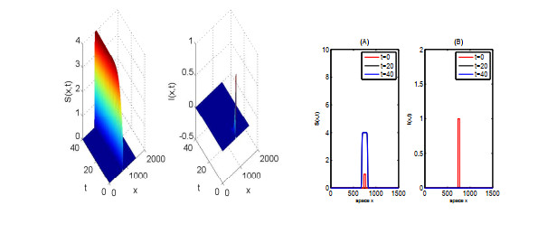
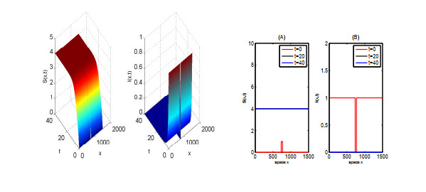
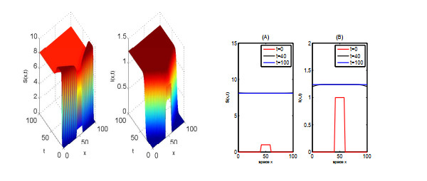
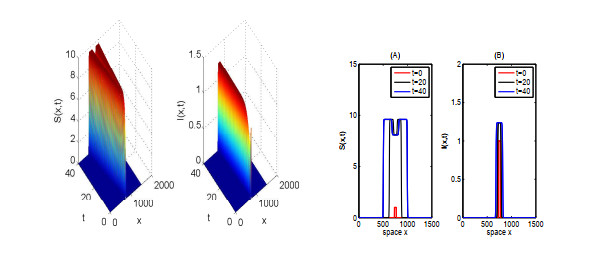
In this paper, we focus on spreading speed of a reaction-diffusion SI epidemic model with vertical transmission, which is a non-monotone system. More specifically, we prove that the solution of the system converges to the disease-free equilibrium as $ t \rightarrow \infty $ if $ R_{0} \leqslant 1 $ and if $ R_0 > 1 $, there exists a critical speed $ c^\diamond > 0 $ such that if $ \|x\| = ct $ with $ c \in (0, c^\diamond) $, the disease is persistent and if $ \|x\| \geqslant ct $ with $ c > c^\diamond $, the infection dies out. Finally, we illustrate the asymptotic behaviour of the solution of the system via numerical simulations.
Citation: Lin Zhao, Haifeng Huo. Spatial propagation for a reaction-diffusion SI epidemic model with vertical transmission[J]. Mathematical Biosciences and Engineering, 2021, 18(5): 6012-6033. doi: 10.3934/mbe.2021301
In this paper, we focus on spreading speed of a reaction-diffusion SI epidemic model with vertical transmission, which is a non-monotone system. More specifically, we prove that the solution of the system converges to the disease-free equilibrium as $ t \rightarrow \infty $ if $ R_{0} \leqslant 1 $ and if $ R_0 > 1 $, there exists a critical speed $ c^\diamond > 0 $ such that if $ \|x\| = ct $ with $ c \in (0, c^\diamond) $, the disease is persistent and if $ \|x\| \geqslant ct $ with $ c > c^\diamond $, the infection dies out. Finally, we illustrate the asymptotic behaviour of the solution of the system via numerical simulations.

| [1] |
A. Ducrot, M. Langlais, P. Magal, Qualitative analysis and travelling wave solutions for the SI model with vertical transmission, Commun. Pure Appl. Anal., 11 (2012), 97-113. doi: 10.3934/cpaa.2012.11.97

|
| [2] | D. G. Aronson, H. F. Weinberger, Nonlinear diffusion in population genetics, combustion, and nerve pulse propagation, in Partial differential equations and related topics, Springer, (1975), 5-49. |
| [3] |
D. G. Aronson, H. F. Weinberger, Multidimensional nonlinear diffusion arising in population dynamics, Adv. Math., 30 (1978), 33-76. doi: 10.1016/0001-8708(78)90130-5
|
| [4] | D. G. Aronson, The asymptotic speed of propagation of a simple epidemic, Nonlinear Diffus., 14 (1977), 1-23. |
| [5] | H. F. Weinberger, Some deterministic models for the spread of genetic and other alterations, in Biological growth and spread, Springer, 1980. |
| [6] |
H. F. Weinberger, Long-time behavior of a class of biological models, SIAM J. Math. Anal., 13 (1982), 353-96. doi: 10.1137/0513028
|
| [7] |
X. Liang, X. Q. Zhao, Spreading speeds and traveling waves for abstract monostable evolution systems, J. Funct. Anal., 259 (2010), 857-903. doi: 10.1016/j.jfa.2010.04.018
|
| [8] |
H. Thieme, X. Q. Zhao, Asymptotic speeds of spread and traveling waves for integral equations and delayed reaction-diffusion models, J. Differ. Equations, 195 (2003), 430-470. doi: 10.1016/S0022-0396(03)00175-X
|
| [9] |
H. Weinberger, On spreading speeds and traveling waves for growth and migration models in a periodic habitat, J. Math. Biol., 45 (2002), 511-548. doi: 10.1007/s00285-002-0169-3
|
| [10] |
H. Weinberger, K. Kawasaki, N. Shigesada, Spreading speeds of spatially periodic integro-difference models for populations with non-monotone recruitment functions, J. Math. Biol., 57 (2008), 387-411. doi: 10.1007/s00285-008-0168-0
|
| [11] |
A. Ducrot, T. Giletti, H. Matano, Spreading speeds for multidimensional reaction-diffusion systems of the prey-predator type, Calc. Var. Partial Differ. Equations, 58 (2019), 1-34. doi: 10.1007/s00526-018-1462-3
|
| [12] |
A. Ducrot, T. Giletti, J. S. Guo, M. Shimojo, Asymptotic spreading speeds for a predator-prey system with two predators and one prey, Nonlinearity, 34 (2021), 669-704. doi: 10.1088/1361-6544/abd289
|
| [13] |
A. Ducrot, Convergence to generalized transition waves for some Holling-Tanner prey-predator reaction-diffusion system, J. Math. Pures Appl., 100 (2013), 1-15. doi: 10.1016/j.matpur.2012.10.009
|
| [14] |
G. Lin, Spreading speeds of a Lotka-Volterra predator-prey system: the role of the predator, Nonlinear Anal., 74 (2011), 2448-2461. doi: 10.1016/j.na.2010.11.046
|
| [15] |
S. Pan, Asymptotic spreading in a Lotka-Volterra predator-prey system, J. Math. Anal. Appl., 407 (2013), 230-236. doi: 10.1016/j.jmaa.2013.05.031
|
| [16] |
Q. Liu, S. Liu, K. Y. Lam, Stacked invasion waves in a competition-diffusion model with three species, J. Differ. Equations, 271 (2021), 665-718. doi: 10.1016/j.jde.2020.09.008
|
| [17] |
A. Ducrot, Spatial propagation for a two component reaction-diffusion system arising in population dynamics, J. Differ. Equations, 260 (2016), 8316-8357. doi: 10.1016/j.jde.2016.02.023
|
| [18] | S. Busenberg, K. Cooke, Vertically transmitted diseases, Models and dynamics, Springer-Verlag, Berlin, 1993. |
| [19] | S. Busenberg, K. L. Cooke, M. A. Pozio, Analysis of a model of vertically transmitted disease, J. Math. Biol., 17 (1983), 30-329. |
| [20] |
A. Ducrot, M. Langlais, P.Magal, Multiple travelling waves for an SI-epidemic model, Netw. Heterog. Media, 8 (2013), 171-190. doi: 10.3934/nhm.2013.8.171
|
| [21] | R. M. Anderson, R. M. May, Infectious Diseases of Humans: Dynamics and Control, Oxford University Press, 1991. |
| [22] |
K. J. Brown, J. Carr, Determinisitic epidemics waves of critical velocity, Math. Proc. Camb. Phil. Soc., 81 (1977), 431-433. doi: 10.1017/S0305004100053494
|
| [23] | O. Diekmann, Thresholds and travelling waves for the geographical spread of infection, J. Math. Biol., 69 (1978), 109-130. |
| [24] |
Y. Hosono, B. Ilyas, Traveling waves for a simple diffusive epdemic model, Math. Models Methods Appl. Sci., 5 (1995), 935-966. doi: 10.1142/S0218202595000504
|
| [25] |
C. Kenndy, R. Aris, Traveling waves in a simple population model invovling growth and death, Bull. Math. Biol., 42 (1980), 397-429. doi: 10.1016/S0092-8240(80)80057-7
|
| [26] | J. D. Murray, Mathematical biology, Springer-Verlag, Berlin, 1989. |
| [27] | L. Rass, J. Radcliffe, Spatial Deterministic Epidemics, American Mathematical Soc., 2003. |
| [28] | S. Cantrell, C. Cosner, S. Ruan Modeling Spatial Spread of Communicable Diseases Involving Animal Hosts, in Spatial Ecology, Chapman and Hall/CRC, (2009), 293-316. |
| [29] |
Z. C. Wang, J. Wu, Traveling waves of a diffusive Kermack-McKendrick epidemic model with nonlocal delayed transmission, Proc. Roy. Soc. A, 466 (2010), 237-261. doi: 10.1098/rspa.2009.0377
|
| [30] |
Z. C. Wang, J. Wu, R. Liu, Traveling waves of the spread of avian influenza, Proc. Amer. Math. Soc., 140 (2012), 3931-3946. doi: 10.1090/S0002-9939-2012-11246-8
|
| [31] |
Z. C. Wang, L. Zhang, X. Q. Zhao, Time periodic traveling waves for a periodic and diffusive SIR epidemic model, J. Dynam. Differ. Equations, 30 (2018), 379-403. doi: 10.1007/s10884-016-9546-2
|
| [32] | R. A. Fisher, The wave of advance of advantageous genes, Ann. Eugenics, 7 (1937), 353-369. |
| [33] | A. N. Kolmogorov, I. G. Petrovsky, N. S. Piskunov, Etude de I'$\acute{e}$quation de la diffusion avec croissance de la quantit$\acute{e}$ de mati$\grave{e}$re et son application $\grave{a}$ un probl$\grave{e}$me biologique, Bull. Univ. Moskow, Ser. Internat., Sec. A, 1 (1937) 1-25. |
| [34] |
A. Ducrot, J. S. Guo, G. Lin, S. Pan, The spreading speed and the minimal wave speed of a predator-prey system with nonlocal dispersal, Z. Angew. Math. Phys., 70 (2019), 1-25. doi: 10.1007/s00033-018-1046-2
|
Figures(5)

Lin Zhao, Haifeng Huo. Spatial propagation for a reaction-diffusion SI epidemic model with vertical transmission[J]. Mathematical Biosciences and Engineering, 2021, 18(5): 6012-6033. doi: 10.3934/mbe.2021301


 DownLoad: