A framework for efficient brain tumor classification using MRI images

Yurong Guan; Muhammad Aamir; Ziaur Rahman; Ammara Ali; Waheed Ahmed Abro; Zaheer Ahmed Dayo; Muhammad Shoaib Bhutta; Zhihua Hu; Yurong Guan; Muhammad Aamir; Ziaur Rahman; Ammara Ali; Waheed Ahmed Abro; Zaheer Ahmed Dayo; Muhammad Shoaib Bhutta; Zhihua Hu

doi:10.3934/mbe.2021292

Mathematical Biosciences and Engineering

2021, Volume 18, Issue 5: 5790-5815. doi: 10.3934/mbe.2021292

Previous Article Next Article

Research article Special Issues

A framework for efficient brain tumor classification using MRI images

1.
Department of Computer Science, Huanggang Normal University, Huangzhou 438000, China
2.
Faculty of Medicine and Health Sciences, Norwegian University of Science and Technology, Norway
3.
Binjiang College, Nanjing University of Information Science & Technology, Wuxi 214105, China
^† The authors contributed equally to this work

Received: 12 May 2021 Accepted: 22 June 2021 Published: 25 June 2021

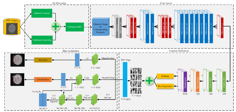
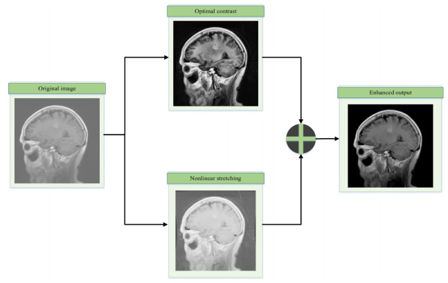
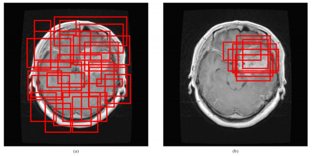
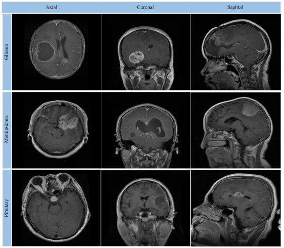
A brain tumor is an abnormal growth of brain cells inside the head, which reduces the patient's survival chance if it is not diagnosed at an earlier stage. Brain tumors vary in size, different in type, irregular in shapes and require distinct therapies for different patients. Manual diagnosis of brain tumors is less efficient, prone to error and time-consuming. Besides, it is a strenuous task, which counts on radiologist experience and proficiency. Therefore, a modern and efficient automated computer-assisted diagnosis (CAD) system is required which may appropriately address the aforementioned problems at high accuracy is presently in need. Aiming to enhance performance and minimise human efforts, in this manuscript, the first brain MRI image is pre-processed to improve its visual quality and increase sample images to avoid over-fitting in the network. Second, the tumor proposals or locations are obtained based on the agglomerative clustering-based method. Third, image proposals and enhanced input image are transferred to backbone architecture for features extraction. Fourth, high-quality image proposals or locations are obtained based on a refinement network, and others are discarded. Next, these refined proposals are aligned to the same size, and finally, transferred to the head network to achieve the desired classification task. The proposed method is a potent tumor grading tool assessed on a publicly available brain tumor dataset. Extensive experiment results show that the proposed method outperformed the existing approaches evaluated on the same dataset and achieved an optimal performance with an overall classification accuracy of 98.04%. Besides, the model yielded the accuracy of 98.17, 98.66, 99.24%, sensitivity (recall) of 96.89, 97.82, 99.24%, and specificity of 98.55, 99.38, 99.25% for Meningioma, Glioma, and Pituitary classes, respectively.

Keywords:

Citation: Yurong Guan, Muhammad Aamir, Ziaur Rahman, Ammara Ali, Waheed Ahmed Abro, Zaheer Ahmed Dayo, Muhammad Shoaib Bhutta, Zhihua Hu. A framework for efficient brain tumor classification using MRI images[J]. Mathematical Biosciences and Engineering, 2021, 18(5): 5790-5815. doi: 10.3934/mbe.2021292

Related Papers:

[1]	Tolga Zaman, Cem Kadilar . Exponential ratio and product type estimators of the mean in stratified two-phase sampling. AIMS Mathematics, 2021, 6(5): 4265-4279. doi: 10.3934/math.2021252
[2]	Khazan Sher, Muhammad Ameeq, Sidra Naz, Basem A. Alkhaleel, Muhammad Muneeb Hassan, Olayan Albalawi . Developing and evaluating efficient estimators for finite population mean in two-phase sampling. AIMS Mathematics, 2025, 10(4): 8907-8925. doi: 10.3934/math.2025408
[3]	Sohaib Ahmad, Sardar Hussain, Muhammad Aamir, Faridoon Khan, Mohammed N Alshahrani, Mohammed Alqawba . Estimation of finite population mean using dual auxiliary variable for non-response using simple random sampling. AIMS Mathematics, 2022, 7(3): 4592-4613. doi: 10.3934/math.2022256
[4]	Yasir Hassan, Muhammad Ismai, Will Murray, Muhammad Qaiser Shahbaz . Efficient estimation combining exponential and ln functions under two phase sampling. AIMS Mathematics, 2020, 5(6): 7605-7623. doi: 10.3934/math.2020486
[5]	Saman Hanif Shahbaz, Aisha Fayomi, Muhammad Qaiser Shahbaz . Estimation of the general population parameter in single- and two-phase sampling. AIMS Mathematics, 2023, 8(7): 14951-14977. doi: 10.3934/math.2023763
[6]	Amber Yousaf Dar, Nadia Saeed, Moustafa Omar Ahmed Abu-Shawiesh, Saman Hanif Shahbaz, Muhammad Qaiser Shahbaz . A new class of ratio type estimators in single- and two-phase sampling. AIMS Mathematics, 2022, 7(8): 14208-14226. doi: 10.3934/math.2022783
[7]	Sanaa Al-Marzouki, Christophe Chesneau, Sohail Akhtar, Jamal Abdul Nasir, Sohaib Ahmad, Sardar Hussain, Farrukh Jamal, Mohammed Elgarhy, M. El-Morshedy . Estimation of finite population mean under PPS in presence of maximum and minimum values. AIMS Mathematics, 2021, 6(5): 5397-5409. doi: 10.3934/math.2021318
[8]	Sohaib Ahmad, Sardar Hussain, Javid Shabbir, Muhammad Aamir, M. El-Morshedy, Zubair Ahmad, Sharifah Alrajhi . Improved generalized class of estimators in estimating the finite population mean using two auxiliary variables under two-stage sampling. AIMS Mathematics, 2022, 7(6): 10609-10624. doi: 10.3934/math.2022592
[9]	Khazan Sher, Muhammad Ameeq, Muhammad Muneeb Hassan, Basem A. Alkhaleel, Sidra Naz, Olyan Albalawi . Novel efficient estimators of finite population mean in stratified random sampling with application. AIMS Mathematics, 2025, 10(3): 5495-5531. doi: 10.3934/math.2025254
[10]	Hleil Alrweili, Fatimah A. Almulhim . Estimation of the finite population mean using extreme values and ranks of the auxiliary variable in two-phase sampling. AIMS Mathematics, 2025, 10(4): 8794-8817. doi: 10.3934/math.2025403

Abstract

1. Introduction

The study of difference equations has long been a cornerstone in the understanding of discrete dynamical systems, with applications spanning fields as diverse as economics, biology, engineering, and time series. Since the 18th century, significant progress has been made in deriving closed-form solutions for certain classes of difference equations and systems (see ^[1,2]). These early contributions laid the foundation for the exploration of solvability in difference equations, a topic still prevalent in modern research. Many classical texts dedicate chapters to the solvability of these systems (see ^[3,4,5]), while recent advancements continue to extend the boundaries of this field (see ^[6,7]). Despite substantial progress, solvable difference equations remain a narrow subset of the broader spectrum of systems, prompting the use of alternative methods to analyze those that lack closed-form solutions (see ^{[4,5,6,7,8,9,10,11,12,13]}).

The quest for solvability often revolves around deriving applicable closed-form formulas, though these can sometimes become exceedingly complex. In such cases, qualitative analysis becomes a more practical approach, providing insights into the system's behavior when explicit solutions are either cumbersome or impossible to obtain (see ^[14]). Nevertheless, when possible, having general solution formulas for new classes of difference equations is invaluable. Many systems, including those involving nonlinearities, can often be transformed into known solvable ones, thereby inheriting their solvability properties. Notable examples include two-dimensional systems studied by Stević, where mathematical transformations were applied to render the systems solvable. For instance, in the work by Stević ^[15], the system of difference equations

$\forall m\geq0, \ \ \ p_{m} = \dfrac{\delta_{m}q_{m-3}}{\alpha_{m}+\beta _{m}q_{m-1}p_{m-2}q_{m-3}}, q_{m} = \dfrac{\delta_{m}^{\prime}p_{m-3}} {\alpha_{m}^{\prime}+\beta_{m}^{\prime}p_{m-1}q_{m-2}p_{m-3}},$

was transformed into a more manageable form, leading to its solvability. Similarly, in another study ^[16], the system

$\forall m\geq0, \ \ \ p_{m} = \dfrac{p_{m-i}q_{m-j}}{\alpha_{m}p_{m-i}+\beta _{m}q_{m-i-j}}, q_{m} = \dfrac{q_{m-i}p_{m-j}}{\alpha_{m}^{\prime} q_{m-i}+\beta_{m}^{\prime}p_{m-i-j}},$

was also successfully transformed into a solvable form. Additionally, in a further study ^[17], a similar approach was used for the system

$\forall m\geq0, \ \ \ p_{m+1} = p_{m}\dfrac{\alpha p_{m}q_{m}+\beta p_{m-1}q_{m-1}}{p_{m-1}q_{m}}, q_{m+1} = \dfrac{p_{m-1}q_{m}^{2}} {\alpha^{\prime}p_{m}q_{m}+\beta^{\prime}p_{m-1}q_{m-1}},$

demonstrating how transformations could simplify the system's structure and allow for deeper insights into its dynamics. These examples underscore the continued relevance of transformation techniques in the analysis of complex dynamic behaviors within difference systems. Such transformations not only render the systems solvable but also provide a clearer understanding of the underlying patterns governing their behavior.

As complex systems continue to emerge in various scientific domains, the need for robust models capable of capturing both the linear and nonlinear behaviors of these systems has grown significantly. Among the various classes of difference equations, three-dimensional systems present a particularly rich area of investigation due to their potential to model real-world phenomena where multiple interacting variables influence the system's evolution. Recent advancements in the study of three-dimensional difference equations have highlighted their critical role in understanding complex dynamical behaviors, especially in systems with nonlinear feedback and interacting variables. For instance, Elsayed et al. ^[18] investigated solutions for nonlinear rational systems, revealing intricate behaviors governed by recursive relations. Similarly, Khaliq et al. ^[19] analyzed exponential difference equations, uncovering stability properties and persistent dynamics in three-dimensional systems. Additionally, Khaliq et al. ^[20] investigated the boundedness nature and persistence, global and local behavior, and rate of convergence of positive solutions of a second-order system of exponential difference equations in three-dimensional systems. Some examples are provided to support their theoretical results. These studies underscore the growing importance of developing analytical and computational tools to tackle the challenges posed by such systems, particularly when closed-form solutions are not readily available. Our paper builds on these contributions by introducing a bilinear transformation approach, providing a novel perspective to study and simplify three-dimensional systems. In this paper, we focus on a specific three-dimensional system of difference equations,

$\begin{align*} \forall m\geq0, \ \ \ \ & p_{m+1} = p_{m}\dfrac{\alpha r_{m}+\beta p_{m-1}q_{m-1} }{p_{m-1}q_{m}}, \\ & q_{m+1} = \dfrac{p_{m-1}q_{m}^{2}}{\gamma r_{m}+\delta p_{m-1}q_{m-1}}, \\ & r_{m+1} = p_{m}q_{m}\dfrac{\varepsilon p_{m}q_{m}+\lambda p_{m-1}q_{m-1} }{\tau p_{m}q_{m}+\sigma p_{m-1}q_{m-1}}, \end{align*}$

(1.a)

where $\alpha, \beta, \gamma, \delta, \varepsilon, \lambda, \tau, \sigma\in \mathbb{R},$ $\alpha^{2}+\beta^{2}\neq0,$ $\gamma^{2}+\delta^{2}\neq0,$ $\varepsilon^{2}+\lambda^{2}\neq0,$ $\tau^{2}+\sigma^{2}\neq0,$ and $p_{0}, q_{0}, p_{-1}, q_{-1}, r_{0}\in\mathbb{R}.$ We employ advanced mathematical transformations and computational tools to unlock a deeper understanding of its dynamics. One of the critical challenges in studying such systems is the complexity of their solutions, especially when nonlinearities and feedback mechanisms are involved. To address this, we introduce a bilinear transformation that simplifies the original system, offering not only a clearer interpretation of its structure but also a more tractable equivalent two-dimensional representation. This approach allows us to focus on essential properties like stability, oscillations, and growth, and how these characteristics evolve under different parameter settings.

Our investigation reveals that this system exhibits rich dynamical behaviors, including oscillatory and stable states, which are significantly influenced by the discriminant of the quadratic polynomial that defines the system. By examining cases of repeated and distinct characteristic roots, we uncover how subtle changes in system parameters can lead to dramatically different outcomes. This insight is particularly valuable for applications in fields like neural networks, where the dynamic interactions between neurons often mirror such complex behaviors.

In the pursuit of developing an advanced model for analyzing the complex interactions within neural systems, we present a sophisticated mathematical framework that integrates recursive equations and nonlinear dynamics. This system aims to explore the evolution of neural signals over time, focusing on how different variables interact to influence overall system stability and activity patterns. By constructing a model based on three critical variables— $p_{m}$ , representing the first neural activity signal, $q_{m}$ , denoting the second neural response, and $r_{m}$ , reflecting the combined influence of both signals—we investigate how fluctuations in these signals impact both short-term dynamics and long-term stability. The recursive nature of the model enables us to track the dynamic behavior of these variables over time, incorporating nonlinear terms to simulate feedback loops characteristic of neural systems. Parameters of our models modulate interactions between the signals, with small constants introduced to ensure numerical stability. Through simulations under varying initial conditions, the model demonstrates how changes in parameter values can lead to markedly different outcomes, such as oscillatory or stable states.

The use of visualizations such as time series, phase diagrams, and frequency analysis complements the theoretical findings, offering insights into the system's behavior across multiple dimensions. These methods are particularly useful in identifying patterns like periodicity, bifurcations, or chaotic behavior, which are critical in understanding how neural systems respond to external stimuli and internal perturbations. This approach not only enhances our understanding of the underlying dynamics in neural networks but also provides a powerful tool for simulating real-world neural behavior. Through this analysis, we aim to bridge the gap between theoretical models and practical applications, offering insights relevant to fields such as neurobiology, artificial neural networks, and systems neuroscience.

The rest of the paper is organized as follows: In Section 2, we address the resolution of the equation system in (1.a). Section 3 focuses on simulation, providing a dynamic analysis of neural activity and system stability using recursive models. Finally, Section 4 concludes the paper with a discussion of the findings and potential directions for future research.

2. Resolution of the equation system in (1.a)

In this section, we turn our attention to the systematic approach required to solve the difference equations outlined in (1.a), subject to specific initial conditions. Consider the sequence $\left(p_{m}, q_{m}, r_{m}\right)$ representing the solution to the system. It is important to highlight that the system may break down and lose its definition if any initial values are zero. To maintain the viability and continuity of the solution, the condition $r_{m+1}q_{m}p_{m}\neq0$ for $m+1\geq0$ must always hold. This ensures the solution is consistent and free from singularities. From this stage onward, we adopt the assumption that $r_{0}q_{-k}p_{-k}\neq0$ for $k\in\left\{ 0, 1\right\}$ . This assumption plays a pivotal role in ensuring the continued existence of a well-defined solution. By securing the integrity of the system through these conditions, we can delve deeper into its dynamics and uncover potential behaviors that the system might exhibit over time.

To ease the analysis and provide a fresh perspective on the system (1.a), we introduce a strategic change of variables. This redefinition aims to simplify the relationships between the variables and allow for clearer insight into the nature of the system. The transformation is expressed as:

$\widehat{p}_{m} = \dfrac{p_{m}q_{m}}{p_{m-1}q_{m-1}}, \text{ }\widehat{r} _{m} = \dfrac{r_{m}}{p_{m-1}q_{m-1}}\text{ for }m\geq0.$

(2.a)

The primary objective of this redefinition is to restructure the system into a more manageable form while retaining its key characteristics. By leveraging these new variables, we simplify the interactions between components, enabling a more straightforward exploration of the system's dynamic behavior. This approach sets the stage for deriving essential properties of the model. To further this simplification, we multiply the corresponding sides of the first and second equations in (1.a), obtaining:

$\begin{align*} \forall m\geq0, \ \ \ & p_{m+1}q_{m+1} = p_{m}q_{m}\dfrac{\alpha r_{m}+\beta p_{m-1}q_{m-1}}{p_{m-1}q_{m}}\dfrac{p_{m-1}q_{m}}{\gamma r_{m}+\delta p_{m-1}q_{m-1}}, \\ & r_{m+1} = p_{m}q_{m}\dfrac{\varepsilon p_{m}q_{m}+\lambda p_{m-1}q_{m-1} }{\tau p_{m}q_{m}+\sigma p_{m-1}q_{m-1}}. \end{align*}$

Simplifying further, we express the system in terms of the transformed variables:

$\begin{align*} \forall m\geq0, \ \ \ \ & \dfrac{p_{m+1}q_{m+1}}{p_{m}q_{m}} = \dfrac{\alpha \dfrac{r_{m}}{p_{m-1}q_{m-1}}+\beta}{\gamma\dfrac{r_{m}}{p_{m-1}q_{m-1} }+\delta}, \\ & \dfrac{r_{m+1}}{p_{m}q_{m}} = \dfrac{\varepsilon\dfrac{p_{m}q_{m}} {p_{m-1}q_{m-1}}+\lambda}{\tau\dfrac{p_{m}q_{m}}{p_{m-1}q_{m-1}}+\sigma}. \end{align*}$

Through this process, the original system (1.a) is recast into the following bilinear form:

$\begin{align*} \forall m\geq0, \widehat{p}_{m+1} = \dfrac{\alpha\widehat{r}_{m}+\beta }{\gamma\widehat{r}_{m}+\delta}, \ \ \ \widehat{r}_{m+1} = \dfrac{\varepsilon \widehat{p}_{m}+\lambda}{\tau\widehat{p}_{m}+\sigma}. \end{align*}$

(2.b)

This new system formulation presents a bilinear structure that simplifies its behavior and makes it easier to analyze. By adopting this approach, we can better understand the interplay between the variables $\widehat{p}_{m}$ and $\widehat{r}_{m}$ . Moreover, this transformation not only aids in solving the system but also provides valuable insights into the long-term dynamics. The bilinear form allows us to examine specific cases where the system may exhibit stability, periodicity, or chaotic behavior, depending on the chosen initial conditions and parameter values.

The nonlinear two-dimensional system of difference equations described in (2.b) was originally introduced by Stević and Tollu ^[17], who demonstrated that the system is solvable by providing a comprehensive method for determining its general solution. Their analysis reveals that certain constraints on the system's parameters are necessary to ensure its solvability. For instance, when $\gamma = 0$ , the first equation in the system (2.b) can be substituted into the second equation, which results in a system characterized by interlacing indices—a structure derived from a bilinear equation. This special case is solvable due to the simplified form of the system. A similar outcome is observed when $\tau = 0$ , which forms a dual case to the one where $\gamma = 0$ . Given these observations, we will operate under the assumption that neither $\gamma$ nor $\tau$ is equal to zero, ensuring the system maintains its nonlinear complexity. Furthermore, to avoid dealing with ill-defined solutions, additional conditions must be met: specifically, we assume $\gamma\widehat{r}_{m}+\delta\neq0$ and $\tau\widehat{p}_{m}+\sigma\neq0$ for all $m$ . These conditions guarantee that the terms in the equations remain valid across iterations. With these assumptions in place, we present the following lemma, as derived from the work of Stević and Tollu ^[17], which lays the groundwork for further analysis of the system.

Lemma 2.1. Let $\alpha, \beta, \gamma, \delta, \varepsilon, \lambda, \tau, \sigma\in\mathbb{R},$ ensuring that the following condition holds: $\gamma\left(\alpha^{2}+\beta^{2}\right) \tau\left(\varepsilon ^{2}+\lambda^{2}\right) \neq0.$ Furthermore, let $\mu_{1}$ and $\mu_{2}$ represent the roots of the quadratic polynomial:

$Q\left( \mu\right) = \mu^{2}-\left( \alpha\varepsilon+\beta\tau +\gamma\lambda+\delta\sigma\right) \mu+\left( \beta\gamma-\alpha \delta\right) \left( \lambda\tau-\varepsilon\sigma\right) .$

Under these conditions, the system of difference equations given in (2.b) admits a closed-form solution. The general solution to this system can be described in two distinct cases, depending on whether the roots $\mu_{1}$ and $\mu_{2}$ coincide or differ.

i. Case $1$ : $\mu_{1} = \mu_{2}.$ In the case where the polynomial $Q\left(\mu\right)$ has a repeated root $\mu_{2}$ , the general solution to the system is given by:

$\begin{align*} \frac{\tau\widehat{p}_{2m}+\sigma}{\tau\widehat{p}_{0}+\sigma} & = \frac{\left( \left( \tau\tfrac{\alpha\tfrac{\varepsilon\widehat{p} _{0}+\lambda}{\tau\widehat{p}_{0}+\sigma}+\beta}{\gamma\tfrac{\varepsilon \widehat{p}_{0}+\lambda}{\tau\widehat{p}_{0}+\sigma}+\delta}+\sigma\right) \left( \gamma\tfrac{\varepsilon\widehat{p}_{0}+\lambda}{\tau\widehat{p} _{0}+\sigma}+\delta\right) -\mu_{2}\right) m+\mu_{2}}{\left( \left( \tau\widehat{p}_{0}+\sigma\right) \left( \gamma\tfrac{\varepsilon\widehat {p}_{0}+\lambda}{\tau\widehat{p}_{0}+\sigma}+\delta\right) -\mu_{2}\right) m+\mu_{2}}, \\ \frac{\left( \gamma\widehat{r}_{0}+\delta\right) }{\mu_{2}}\left( \tau\widehat{p}_{2m+1}+\sigma\right) & = \frac{\left( \left( \tau \tfrac{\alpha\widehat{r}_{0}+\beta}{\gamma\widehat{r}_{0}+\delta} +\sigma\right) \left( \gamma\widehat{r}_{0}+\delta\right) -\mu_{2}\right) \left( 1+m\right) +\mu_{2}}{\left( \left( \tau\tfrac{\alpha\widehat{r} _{0}+\beta}{\gamma\widehat{r}_{0}+\delta}+\sigma\right) \left( \gamma \tfrac{\varepsilon\tfrac{\alpha\widehat{r}_{0}+\beta}{\gamma\widehat{r} _{0}+\delta}+\lambda}{\tau\tfrac{\alpha\widehat{r}_{0}+\beta}{\gamma \widehat{r}_{0}+\delta}+\sigma}+\delta\right) -\mu_{2}\right) m+\mu_{2}}, \\ \frac{\gamma\widehat{r}_{2m}+\delta}{\gamma\widehat{r}_{0}+\delta} & = \frac{\left( \left( \tau\tfrac{\alpha\widehat{r}_{0}+\beta}{\gamma \widehat{r}_{0}+\delta}+\sigma\right) \left( \gamma\tfrac{\varepsilon \tfrac{\alpha\widehat{r}_{0}+\beta}{\gamma\widehat{r}_{0}+\delta}+\lambda }{\tau\tfrac{\alpha\widehat{r}_{0}+\beta}{\gamma\widehat{r}_{0}+\delta} +\sigma}+\delta\right) -\mu_{2}\right) m+\mu_{2}}{\left( \left( \tau \tfrac{\alpha\widehat{r}_{0}+\beta}{\gamma\widehat{r}_{0}+\delta} +\sigma\right) \left( \gamma\widehat{r}_{0}+\delta\right) -\mu_{2}\right) m+\mu_{2}}, \\ \frac{\left( \tau\widehat{p}_{0}+\sigma\right) }{\mu_{2}}\left( \gamma\widehat{r}_{2m+1}+\delta\right) & = \frac{\left( \left( \tau\widehat{p}_{0}+\sigma\right) \left( \gamma\tfrac{\varepsilon\widehat {p}_{0}+\lambda}{\tau\widehat{p}_{0}+\sigma}+\delta\right) -\mu_{2}\right) \left( 1+m\right) +\mu_{2}}{\left( \left( \tau\tfrac{\alpha\tfrac {\varepsilon\widehat{p}_{0}+\lambda}{\tau\widehat{p}_{0}+\sigma}+\beta} {\gamma\tfrac{\varepsilon\widehat{p}_{0}+\lambda}{\tau\widehat{p}_{0}+\sigma }+\delta}+\sigma\right) \left( \gamma\tfrac{\varepsilon\widehat{p} _{0}+\lambda}{\tau\widehat{p}_{0}+\sigma}+\delta\right) -\mu_{2}\right) m+\mu_{2}}. \end{align*}$

This solution highlights how the behavior of the system evolves in the case of a repeated root, where the sequences $\left(\widehat{p}_{m}\right)$ and $\left(\widehat{r}_{m}\right)$ depend on both the initial values and the root $\mu_{2}$ , with a linear relationship to the index m.

ii. Case $2$ : $\mu_{1}\neq\mu_{2}.$ When the roots $\mu_{1}$ and $\mu_{2}$ are distinct, the general solution takes a different form, reflecting the more complex interplay between the two roots:

$\begin{align*} \frac{\tau\widehat{p}_{2m}+\sigma}{\tau\widehat{p}_{0}+\sigma} & = \frac{\left( \tau\tfrac{\alpha\tfrac{\varepsilon\widehat{p}_{0}+\lambda }{\tau\widehat{p}_{0}+\sigma}+\beta}{\gamma\tfrac{\varepsilon\widehat{p} _{0}+\lambda}{\tau\widehat{p}_{0}+\sigma}+\delta}+\sigma\right) \left( \gamma\tfrac{\varepsilon\widehat{p}_{0}+\lambda}{\tau\widehat{p}_{0}+\sigma }+\delta\right) \left( \mu_{1}^{m}-\mu_{2}^{m}\right) +\mu_{1}\mu _{2}\left( \mu_{2}^{m-1}-\mu_{1}^{m-1}\right) }{\left( \tau\widehat{p} _{0}+\sigma\right) \left( \gamma\tfrac{\varepsilon\widehat{p}_{0}+\lambda }{\tau\widehat{p}_{0}+\sigma}+\delta\right) \left( \mu_{1}^{m}-\mu_{2} ^{m}\right) +\mu_{1}\mu_{2}\left( \mu_{2}^{m-1}-\mu_{1}^{m-1}\right) }, \\ \left( \gamma\widehat{r}_{0}+\delta\right) \left( \tau\widehat{p} _{2m+1}+\sigma\right) & = \frac{\left( \tau\tfrac{\alpha\widehat{r} _{0}+\beta}{\gamma\widehat{r}_{0}+\delta}+\sigma\right) \left( \gamma\widehat{r}_{0}+\delta\right) \left( \mu_{1}^{m+1}-\mu_{2} ^{m+1}\right) +\mu_{1}\mu_{2}\left( \mu_{2}^{m}-\mu_{1}^{m}\right) }{\left( \tau\tfrac{\alpha\widehat{r}_{0}+\beta}{\gamma\widehat{r}_{0} +\delta}+\sigma\right) \left( \gamma\tfrac{\varepsilon\tfrac{\alpha \widehat{r}_{0}+\beta}{\gamma\widehat{r}_{0}+\delta}+\lambda}{\tau \tfrac{\alpha\widehat{r}_{0}+\beta}{\gamma\widehat{r}_{0}+\delta}+\sigma }+\delta\right) \left( \mu_{1}^{m}-\mu_{2}^{m}\right) +\mu_{1}\mu _{2}\left( \mu_{2}^{m-1}-\mu_{1}^{m-1}\right) }, \\ \frac{\gamma\widehat{r}_{2m}+\delta}{\gamma\widehat{r}_{0}+\delta} & = \frac{\left( \tau\tfrac{\alpha\widehat{r}_{0}+\beta}{\gamma\widehat{r} _{0}+\delta}+\sigma\right) \left( \gamma\tfrac{\varepsilon\tfrac {\alpha\widehat{r}_{0}+\beta}{\gamma\widehat{r}_{0}+\delta}+\lambda} {\tau\tfrac{\alpha\widehat{r}_{0}+\beta}{\gamma\widehat{r}_{0}+\delta}+\sigma }+\delta\right) \left( \mu_{1}^{m}-\mu_{2}^{m}\right) +\mu_{1}\mu _{2}\left( \mu_{2}^{m-1}-\mu_{1}^{m-1}\right) }{\left( \tau\tfrac {\alpha\widehat{r}_{0}+\beta}{\gamma\widehat{r}_{0}+\delta}+\sigma\right) \left( \gamma\widehat{r}_{0}+\delta\right) \left( \mu_{1}^{m}-\mu_{2} ^{m}\right) +\mu_{1}\mu_{2}\left( \mu_{2}^{m-1}-\mu_{1}^{m-1}\right) }, \\ \left( \tau\widehat{p}_{0}+\sigma\right) \left( \gamma\widehat{r} _{2m+1}+\delta\right) & = \frac{\left( \tau\widehat{p}_{0}+\sigma\right) \left( \gamma\tfrac{\varepsilon\widehat{p}_{0}+\lambda}{\tau\widehat{p} _{0}+\sigma}+\delta\right) \left( \mu_{1}^{m+1}-\mu_{2}^{m+1}\right) +\mu_{1}\mu_{2}\left( \mu_{2}^{m}-\mu_{1}^{m}\right) }{\left( \tau \tfrac{\alpha\tfrac{\varepsilon\widehat{p}_{0}+\lambda}{\tau\widehat{p} _{0}+\sigma}+\beta}{\gamma\tfrac{\varepsilon\widehat{p}_{0}+\lambda} {\tau\widehat{p}_{0}+\sigma}+\delta}+\sigma\right) \left( \gamma \tfrac{\varepsilon\widehat{p}_{0}+\lambda}{\tau\widehat{p}_{0}+\sigma} +\delta\right) \left( \mu_{1}^{m}-\mu_{2}^{m}\right) +\mu_{1}\mu_{2}\left( \mu_{2}^{m-1}-\mu_{1}^{m-1}\right) }. \end{align*}$

This form of the solution captures the intricate dynamics of the system when the two roots differ. The system exhibits oscillatory or exponential behavior depending on the magnitude and sign of $\mu_{1}$ and $\mu_{2}$ , reflecting the underlying complexity of the difference equations.

Remark 2.1. In certain cases, when specific relationships hold among the parameters of the system, simpler solutions can be derived. Specifically, if $\beta\gamma = \alpha\delta$ or $\lambda\tau = \varepsilon\sigma$ , the system (2.b) can be significantly simplified. When $\beta\gamma = \alpha\delta$ , the system reduces to a straightforward form where the sequences $\left(\widehat{p}_{m}\right)$ and $\left(\widehat{r} _{m}\right)$ stabilize to constant values. In this case, we have the following:

$\forall m\geq0, \widehat{p}_{m} = \left\{ \begin{array} [c]{ll} \dfrac{\alpha}{\gamma} & if\ \gamma\neq0 \\ \dfrac{\beta}{\delta} & if\ \delta\neq0 \end{array} \ \right. , \ \ \ \widehat{r}_{m} = \left\{ \begin{array}{ll} \dfrac{\alpha\varepsilon+\gamma\lambda}{\alpha\tau+\gamma\sigma} & if\ \gamma\neq0 \\ \dfrac{\beta\varepsilon+\delta\lambda}{\beta\tau+\delta\sigma} & if \ \delta\neq0 \end{array} \ \right. .$

Similarly, if $\lambda\tau = \varepsilon\sigma$ , the sequences $\left(\widehat{p}_{m}\right)$ and $\left(\widehat{r}_{m}\right)$ are also reduced to constant expressions, but with a different set of parameters governing their values:

$\forall m\geq0, \widehat{p}_{m} = \left\{ \begin{array}{ll} \dfrac{\varepsilon\alpha+\tau\beta}{\varepsilon\gamma+\tau\delta} & if \ \tau\neq0 \\ \dfrac{\lambda\alpha+\sigma\beta}{\lambda\gamma+\sigma\delta} & if \ \sigma\neq0 \end{array} \ \right. , \ \ \ \widehat{r}_{m} = \left\{ \begin{array}{ll} \dfrac{\varepsilon}{\tau} & if \ \tau\neq0 \\ \dfrac{\lambda}{\sigma} & if \ \sigma\neq0 \end{array} \ \right. .$

These simplified cases are particularly useful when certain parameter combinations lead to degeneracies in the system, enabling us to derive constant sequences for $\left(\widehat{p}_{m}\right)$ and $\left(\widehat{r}_{m}\right)$ , which can make further analysis much more manageable.

Remark 2.2. Additionally, from the quadratic polynomial $Q\left(\mu\right)$ , a necessary and sufficient condition for the system to have distinct roots $\mu_{1}$ and $\mu_{2}$ is that the following inequality holds:

$\dfrac{\left( \alpha\varepsilon+\beta\tau+\gamma\lambda+\delta\sigma\right) ^{2}}{\left( \beta\gamma-\alpha\delta\right) \left( \lambda\tau -\varepsilon\sigma\right) }\neq4.$

(2.c)

This condition ensures that the system avoids critical cases where the roots $\mu_{1}$ and $\mu_{2}$ coincide, thereby maintaining the generality of the solution structure.

According to Lemma 2.1, we derive the closed-form expressions for the solutions of system (1.a). From these solutions, we can formulate the following theorem.

Theorem 2.1. Let $\alpha, \beta, \gamma, \delta, \varepsilon, \lambda, \tau, \sigma\in\mathbb{R},$ where the condition $\gamma\left(\alpha^{2}+\beta^{2}\right) \tau\left(\varepsilon^{2}+\lambda^{2}\right) \neq0$ holds $.$ Under these parameters, the system of difference equations presented in (2.b) admits a general closed-form solution. The solution to this system is expressed in two distinct cases, based on whether the roots $\mu_{1}$ and $\mu_{2}$ are identical or distinct.

i. Case $1$ : Under the assumption specified in (2.c), the general solution to the system is:

$\begin{align*} p_{2m+s} & = p_{0}\tfrac{\alpha r_{0}+\beta p_{-1}q_{-1}}{p_{-1}q_{0} }\left\{ { \prod\limits_{l = 1}^{m-1+s}} \frac{q_{0}}{\gamma}\left( \alpha\left( \gamma\tfrac{r_{0}}{p_{-1}q_{-1} }+\delta\right) \left( \left( \tau\tfrac{\alpha r_{0}+\beta p_{-1}q_{-1} }{\gamma r_{0}+\delta p_{-1}q_{-1}}+\sigma\right) \left( \gamma \tfrac{\varepsilon\tfrac{\alpha r_{0}+\beta p_{-1}q_{-1}}{\gamma r_{0}+\delta p_{-1}q_{-1}}+\lambda}{\tau\tfrac{\alpha r_{0}+\beta p_{-1}q_{-1}}{\gamma r_{0}+\delta p_{-1}q_{-1}}+\sigma}+\delta\right) \right. \right. \right. \\ & \times\left. \left( \mu_{1}^{l}-\mu_{2}^{l}\right) +\mu_{1}\mu _{2}\left( \mu_{2}^{l-1}-\mu_{1}^{l-1}\right) \right) \left( \left( \tau\tfrac{\alpha r_{0}+\beta p_{-1}q_{-1}}{\gamma r_{0}+\delta p_{-1}q_{-1} }+\sigma\right) \left( \gamma\tfrac{r_{0}}{p_{-1}q_{-1}}+\delta\right) \left( \mu_{1}^{l}-\mu_{2}^{l}\right) \right. \\ & +\left. \left. \left. \mu_{1}\mu_{2}\left( \mu_{2}^{l-1}-\mu_{1} ^{l-1}\right) \right) ^{-1}+\beta\gamma-\alpha\delta\right) \right\} \times\left\{ { \prod\limits_{l = 1}^{m}} \frac{q_{0}}{\gamma}\left( \tfrac{\alpha}{\left( \tau\tfrac{p_{0}q_{0} }{p_{-1}q_{-1}}+\sigma\right) }\right. \right. \left( \left( \tau \tfrac{p_{0}q_{0}}{p_{-1}q_{-1}}+\sigma\right) \right. \\ & \times\left. \left( \gamma\tfrac{\varepsilon p_{0}q_{0}+\lambda p_{-1}q_{-1}}{\tau p_{0}q_{0}+\sigma p_{-1}q_{-1}}+\delta\right) \left( \mu_{1}^{l}-\mu_{2}^{l}\right) +\mu_{1}\mu_{2}\left( \mu_{2}^{l-1}-\mu _{1}^{l-1}\right) \right) \left( \left( \tau\tfrac{\alpha\tfrac {\varepsilon p_{0}q_{0}+\lambda p_{-1}q_{-1}}{\tau p_{0}q_{0}+\sigma p_{-1}q_{-1}}+\beta}{\gamma\tfrac{\varepsilon p_{0}q_{0}+\lambda p_{-1}q_{-1} }{\tau p_{0}q_{0}+\sigma p_{-1}q_{-1}}+\delta}+\sigma\right) \right. \\ & \times\left. \left. \left. \left( \gamma\tfrac{\varepsilon p_{0} q_{0}+\lambda p_{-1}q_{-1}}{\tau p_{0}q_{0}+\sigma p_{-1}q_{-1}} +\delta\right) \left( \mu_{1}^{l-1}-\mu_{2}^{l-1}\right) +\mu_{1}\mu _{2}\left( \mu_{2}^{l-2}-\mu_{1}^{l-2}\right) \right) ^{-1}-\alpha \delta+\beta\gamma\right) \right\} \\ & \times { \prod\limits_{l = 2}^{2m+s}} \left( \left\{ { \prod\limits_{k = 1}^{\left[ \frac{l}{2}\right] -1}} \left( \gamma\tfrac{r_{0}}{p_{-1}q_{-1}}+\delta\right) \left( \left( \tau\tfrac{\alpha r_{0}+\beta p_{-1}q_{-1}}{\gamma r_{0}+\delta p_{-1}q_{-1} }+\sigma\right) \left( \gamma\tfrac{\varepsilon\tfrac{\alpha r_{0}+\beta p_{-1}q_{-1}}{\gamma r_{0}+\delta p_{-1}q_{-1}}+\lambda}{\tau\tfrac{\alpha r_{0}+\beta p_{-1}q_{-1}}{\gamma r_{0}+\delta p_{-1}q_{-1}}+\sigma} +\delta\right) \right. \right. \right. \left( \mu_{1}^{k}-\mu_{2} ^{k}\right) \\ & \left. \left. +\mu_{1}\mu_{2}\left( \mu_{2}^{k-1}-\mu_{1}^{k-1}\right) \right) \left( \left( \tau\tfrac{\alpha r_{0}+\beta p_{-1}q_{-1}}{\gamma r_{0}+\delta p_{-1}q_{-1}}+\sigma\right) \left( \gamma\tfrac{r_{0}} {p_{-1}q_{-1}}+\delta\right) \left( \mu_{1}^{k}-\mu_{2}^{k}\right) +\mu _{1}\mu_{2}\left( \mu_{2}^{m-1}-\mu_{1}^{k-1}\right) \right) ^{-1}\right\} \\ & \times\left\{ { \prod\limits_{k = 1}^{\left[ \frac{l-1}{2}\right] }} \dfrac{1}{\left( \tau\tfrac{p_{0}q_{0}}{p_{-1}q_{-1}}+\sigma\right) }\right. \left( \left( \tau\tfrac{p_{0}q_{0}}{p_{-1}q_{-1}}+\sigma\right) \left( \gamma\tfrac{\varepsilon p_{0}q_{0}+\lambda p_{-1}q_{-1}}{\tau p_{0}q_{0}+\sigma p_{-1}q_{-1}}+\delta\right) \left( \mu_{1}^{k}-\mu_{2} ^{k}\right) \mu_{1}\mu_{2}\left( \mu_{2}^{k-1}-\mu_{1}^{k-1}\right) \right) \\ & \times\left. \left( \left( \tau\tfrac{\alpha\tfrac{\varepsilon p_{0}q_{0}+\lambda p_{-1}q_{-1}}{\tau p_{0}q_{0}+\sigma p_{-1}q_{-1}}+\beta }{\gamma\tfrac{\varepsilon p_{0}q_{0}+\lambda p_{-1}q_{-1}}{\tau p_{0} q_{0}+\sigma p_{-1}q_{-1}}+\delta}+\sigma\right) \left( \gamma \tfrac{\varepsilon p_{0}q_{0}+\lambda p_{-1}q_{-1}}{\tau p_{0}q_{0}+\sigma p_{-1}q_{-1}}+\delta\right) \left( \mu_{1}^{k-1}-\mu_{2}^{k-1}\right) +\mu_{1}\mu_{2}\left( \mu_{2}^{k-2}-\mu_{1}^{k-2}\right) \right) ^{-1}\right\} \\ & \left. \left/ \tfrac{p_{-1}q_{0}^{2}}{\gamma r_{0}+\delta p_{-1}q_{-1} }\right. \right) , \end{align*}$

$\begin{align*} q_{2m+s} & = q_{0}\left( \tfrac{p_{-1}q_{0}^{2}}{\gamma r_{0}+\delta p_{-1}q_{-1}}\right) ^{2m+s}\left/ { \prod\limits_{l = 1}^{2m+s}} \left( q_{0}\left\{ { \prod\limits_{k = 1}^{\left[ \frac{l-1}{2}\right] }} \left( \gamma\tfrac{r_{0}}{p_{-1}q_{-1}}+\delta\right) \left( \left( \tau\tfrac{\alpha r_{0}+\beta p_{-1}q_{-1}}{\gamma r_{0}+\delta p_{-1}q_{-1} }+\sigma\right) \right. \right. \right. \right. \\ & \times\left. \left( \gamma\tfrac{\varepsilon\tfrac{\alpha r_{0}+\beta p_{-1}q_{-1}}{\gamma r_{0}+\delta p_{-1}q_{-1}}+\lambda}{\tau\tfrac{\alpha r_{0}+\beta p_{-1}q_{-1}}{\gamma r_{0}+\delta p_{-1}q_{-1}}+\sigma} +\delta\right) \left( \mu_{1}^{k}-\mu_{2}^{k}\right) +\mu_{1}\mu_{2}\left( \mu_{2}^{k-1}-\mu_{1}^{k-1}\right) \right) \left( \left( \tau\tfrac{\alpha r_{0}+\beta p_{-1}q_{-1}}{\gamma r_{0}+\delta p_{-1}q_{-1}}+\sigma\right) \left( \gamma\tfrac{r_{0}}{p_{-1}q_{-1}}+\delta\right) \right. \\ & \left. \left. \times\left( \mu_{1}^{k}-\mu_{2}^{k}\right) +\mu_{1} \mu_{2}\left( \mu_{2}^{m-1}-\mu_{1}^{k-1}\right) \right) ^{-1}\right\} \times\left\{ { \prod\limits_{k = 1}^{\left[ \frac{l}{2}\right] }} \dfrac{1}{\left( \tau\tfrac{p_{0}q_{0}}{p_{-1}q_{-1}}+\sigma\right) }\left( \left( \tau\tfrac{p_{0}q_{0}}{p_{-1}q_{-1}}+\sigma\right) \right. \right. \\ & \left. \times\left( \gamma\tfrac{\varepsilon p_{0}q_{0}+\lambda p_{-1}q_{-1}}{\tau p_{0}q_{0}+\sigma p_{-1}q_{-1}}+\delta\right) \left( \mu_{1}^{k}-\mu_{2}^{k}\right) +\mu_{1}\mu_{2}\left( \mu_{2}^{k-1}-\mu _{1}^{k-1}\right) \right) \left( \left( \tau\tfrac{\alpha\tfrac {\varepsilon p_{0}q_{0}+\lambda p_{-1}q_{-1}}{\tau p_{0}q_{0}+\sigma p_{-1}q_{-1}}+\beta}{\gamma\tfrac{\varepsilon p_{0}q_{0}+\lambda p_{-1}q_{-1} }{\tau p_{0}q_{0}+\sigma p_{-1}q_{-1}}+\delta}+\sigma\right) \right. \\ & \left. \left. \left. \times\left( \gamma\tfrac{\varepsilon p_{0} q_{0}+\lambda p_{-1}q_{-1}}{\tau p_{0}q_{0}+\sigma p_{-1}q_{-1}} +\delta\right) \left( \mu_{1}^{k-1}-\mu_{2}^{k-1}\right) +\mu_{1}\mu _{2}\left( \mu_{2}^{k-2}-\mu_{1}^{k-2}\right) \right) ^{-1}\right\} \right) , \end{align*}$

$\begin{align*} r_{2m} & = p_{2m-1}q_{2m-1}\left( \left( \tfrac{r_{0}}{p_{-1}q_{-1}} +\frac{\delta}{\gamma}\right) \left( \left( \tau\tfrac{\alpha r_{0}+\beta p_{-1}q_{-1}}{\gamma r_{0}+\delta p_{-1}q_{-1}}+\sigma\right) \left( \gamma\tfrac{\varepsilon\tfrac{\alpha r_{0}+\beta p_{-1}q_{-1}}{\gamma r_{0}+\delta p_{-1}q_{-1}}+\lambda}{\tau\tfrac{\alpha r_{0}+\beta p_{-1} q_{-1}}{\gamma r_{0}+\delta p_{-1}q_{-1}}+\sigma}+\delta\right) \left( \mu_{1}^{m}-\mu_{2}^{m}\right) \right. \right. \\ & +\left. \mu_{1}\mu_{2}\left( \mu_{2}^{m-1}-\mu_{1}^{m-1}\right) \right) \left( \left( \tau\tfrac{\alpha r_{0}+\beta p_{-1}q_{-1}}{\gamma r_{0}+\delta p_{-1}q_{-1}}+\sigma\right) \left( \gamma\tfrac{r_{0}} {p_{-1}q_{-1}}+\delta\right) \left( \mu_{1}^{m}-\mu_{2}^{m}\right) +\mu _{1}\mu_{2}\right. \\ & \times\left. \left. \left( \mu_{2}^{m-1}-\mu_{1}^{m-1}\right) \right) ^{-1}-\frac{\delta}{\gamma}\right) , \end{align*}$

$\begin{align*} r_{2m+1} & = p_{2m}q_{2m}\left( \dfrac{1}{\gamma\left( \tau\tfrac {p_{0}q_{0}}{p_{-1}q_{-1}}+\sigma\right) }\right. \left( \left( \tau \tfrac{p_{0}q_{0}}{p_{-1}q_{-1}}+\sigma\right) \left( \gamma\tfrac {\varepsilon p_{0}q_{0}+\lambda p_{-1}q_{-1}}{\tau p_{0}q_{0}+\sigma p_{-1}q_{-1}}+\delta\right) \left( \mu_{1}^{m+1}-\mu_{2}^{m+1}\right) \right. \\ & +\left. \mu_{1}\mu_{2}\left( \mu_{2}^{m}-\mu_{1}^{m}\right) \right) \left( \left( \tau\tfrac{\alpha\tfrac{\varepsilon p_{0}q_{0}+\lambda p_{-1}q_{-1}}{\tau p_{0}q_{0}+\sigma p_{-1}q_{-1}}+\beta}{\gamma \tfrac{\varepsilon p_{0}q_{0}+\lambda p_{-1}q_{-1}}{\tau p_{0}q_{0}+\sigma p_{-1}q_{-1}}+\delta}+\sigma\right) \left( \gamma\tfrac{\varepsilon p_{0}q_{0}+\lambda p_{-1}q_{-1}}{\tau p_{0}q_{0}+\sigma p_{-1}q_{-1}} +\delta\right) \left( \mu_{1}^{m}-\mu_{2}^{m}\right) \right. \\ & \left. \left. +\mu_{1}\mu_{2}\left( \mu_{2}^{m-1}-\mu_{1}^{m-1}\right) \right) ^{-1}-\frac{\delta}{\gamma}\right) , \end{align*}$

for $s\in\left\{ 0, 1\right\},$ and $m\geq0.$

ii. Case $2$ : When the assumption in (2.c) is not satisfied, the general solution becomes:

$\begin{align*} p_{2m+s} & = p_{0}\tfrac{\alpha r_{0}+\beta p_{-1}q_{-1}}{p_{-1}q_{0} }\left\{ { \prod\limits_{l = 1}^{m-1+s}} \frac{q_{0}}{\gamma}\left( \alpha\left( \gamma\tfrac{r_{0}}{p_{-1}q_{-1} }+\delta\right) \left( \left( \left( \left( \tau\tfrac{\alpha r_{0}+\beta p_{-1}q_{-1}}{\gamma r_{0}+\delta p_{-1}q_{-1}}+\sigma\right) \left( \gamma\tfrac{\varepsilon\tfrac{\alpha r_{0}+\beta p_{-1}q_{-1}}{\gamma r_{0}+\delta p_{-1}q_{-1}}+\lambda}{\tau\tfrac{\alpha r_{0}+\beta p_{-1} q_{-1}}{\gamma r_{0}+\delta p_{-1}q_{-1}}+\sigma}+\delta\right) \right. \right. \right. \right. \right. \\ & \left. \left. \left. \left. -\mu_{2}\right) l+\mu_{2}\right) \left( \left( \left( \tau\tfrac{\alpha r_{0}+\beta p_{-1}q_{-1}}{\gamma r_{0}+\delta p_{-1}q_{-1}}+\sigma\right) \left( \gamma\tfrac{r_{0}} {p_{-1}q_{-1}}+\delta\right) -\mu_{2}\right) l+\mu_{2}\right) ^{-1} -\alpha\delta+\beta\gamma\right) \right\} \\ & \times\left\{ { \prod\limits_{l = 1}^{m}} \frac{q_{0}}{\gamma}\left( \tfrac{\alpha\mu_{2}}{\left( \tau\tfrac {p_{0}q_{0}}{p_{-1}q_{-1}}+\sigma\right) }\right. \right. \left( \left( \left( \tau\tfrac{p_{0}q_{0}}{p_{-1}q_{-1}}+\sigma\right) \left( \gamma\tfrac{\varepsilon p_{0}q_{0}+\lambda p_{-1}q_{-1}}{\tau p_{0} q_{0}+\sigma p_{-1}q_{-1}}+\delta\right) -\mu_{2}\right) l+\mu_{2}\right) \\ & \times\left. \left. \left( \left( \left( \tau\dfrac{\alpha \tfrac{\varepsilon p_{0}q_{0}+\lambda p_{-1}q_{-1}}{\tau p_{0}q_{0}+\sigma p_{-1}q_{-1}}+\beta}{\gamma\tfrac{\varepsilon p_{0}q_{0}+\lambda p_{-1}q_{-1} }{\tau p_{0}q_{0}+\sigma p_{-1}q_{-1}}+\delta}+\sigma\right) \left( \gamma\tfrac{\varepsilon p_{0}q_{0}+\lambda p_{-1}q_{-1}}{\tau p_{0} q_{0}+\sigma p_{-1}q_{-1}}+\delta\right) -\mu_{2}\right) \left( l-1\right) +\mu_{2}\right) ^{-1}-\alpha\delta+\beta\gamma\right) \right\} \\ & \times { \prod\limits_{l = 2}^{2m+s}} \left( \left\{ { \prod\limits_{k = 1}^{\left[ \frac{l}{2}\right] -1}} \left( \gamma\tfrac{r_{0}}{p_{-1}q_{-1}}+\delta\right) \left( \left( \left( \tau\tfrac{\alpha r_{0}+\beta p_{-1}q_{-1}}{\gamma r_{0}+\delta p_{-1}q_{-1}}+\sigma\right) \left( \gamma\tfrac{\varepsilon\tfrac{\alpha r_{0}+\beta p_{-1}q_{-1}}{\gamma r_{0}+\delta p_{-1}q_{-1}}+\lambda} {\tau\tfrac{\alpha r_{0}+\beta p_{-1}q_{-1}}{\gamma r_{0}+\delta p_{-1}q_{-1} }+\sigma}+\delta\right) -\mu_{2}\right) k+\mu_{2}\right) \right. \right. \\ & \times\left. \left( \left( \left( \tau\tfrac{\alpha r_{0}+\beta p_{-1}q_{-1}}{\gamma r_{0}+\delta p_{-1}q_{-1}}+\sigma\right) \left( \gamma\tfrac{r_{0}}{p_{-1}q_{-1}}+\delta\right) -\mu_{2}\right) k+\mu _{2}\right) ^{-1}\right\} \times\left\{ { \prod\limits_{k = 1}^{\left[ \frac{l-1}{2}\right] }} \tfrac{\mu_{2}}{\left( \tau\tfrac{p_{0}q_{0}}{p_{-1}q_{-1}}+\sigma\right) }\right. \left( \left( \left( \tau\tfrac{p_{0}q_{0}}{p_{-1}q_{-1}} +\sigma\right) \right. \right. \\ & \times\left. \left. \left( \gamma\tfrac{\varepsilon p_{0}q_{0}+\lambda p_{-1}q_{-1}}{\tau p_{0}q_{0}+\sigma p_{-1}q_{-1}}+\delta\right) -\mu _{2}\right) k+\mu_{2}\right) \left( \left( \left( \tau\tfrac{\alpha \tfrac{\varepsilon p_{0}q_{0}+\lambda p_{-1}q_{-1}}{\tau p_{0}q_{0}+\sigma p_{-1}q_{-1}}+\beta}{\gamma\tfrac{\varepsilon p_{0}q_{0}+\lambda p_{-1}q_{-1} }{\tau p_{0}q_{0}+\sigma p_{-1}q_{-1}}+\delta}+\sigma\right) \left( \gamma\tfrac{\varepsilon p_{0}q_{0}+\lambda p_{-1}q_{-1}}{\tau p_{0} q_{0}+\sigma p_{-1}q_{-1}}+\delta\right) \right. \right. \\ & \left. \left. \left. \left. -\mu_{2}\right) \left( k-1\right) +\mu_{2}\right) \right\} \left/ \tfrac{p_{-1}q_{0}^{2}}{\gamma r_{0}+\delta p_{-1}q_{-1}}\right. \right) , \end{align*}$

$\begin{align*} q_{2m+s} & = q_{0}\left( \tfrac{p_{-1}q_{0}^{2}}{\gamma r_{0}+\delta p_{-1}q_{-1}}\right) ^{2m+s}\left/ { \prod\limits_{l = 1}^{2m+s}} \left( q_{0}\left\{ { \prod\limits_{k = 1}^{\left[ \frac{l-1}{2}\right] }} \left( \gamma\tfrac{r_{0}}{p_{-1}q_{-1}}+\delta\right) \left( \left( \left( \tau\tfrac{\alpha r_{0}+\beta p_{-1}q_{-1}}{\gamma r_{0}+\delta p_{-1}q_{-1}}+\sigma\right) \right. \right. \right. \right. \right. \\ & \times\left. \left. \left. \left( \gamma\tfrac{\varepsilon\tfrac{\alpha r_{0}+\beta p_{-1}q_{-1}}{\gamma r_{0}+\delta p_{-1}q_{-1}}+\lambda} {\tau\tfrac{\alpha r_{0}+\beta p_{-1}q_{-1}}{\gamma r_{0}+\delta p_{-1}q_{-1} }+\sigma}+\delta\right) -\mu_{2}\right) \right) k+\mu_{2}\right) \left( \left( \left( \tau\tfrac{\alpha r_{0}+\beta p_{-1}q_{-1}}{\gamma r_{0}+\delta p_{-1}q_{-1}}+\sigma\right) \left( \gamma\tfrac{r_{0}} {p_{-1}q_{-1}}+\delta\right) \right. \right. \\ & \left. \left. \left. -\mu_{2}\right) k+\mu_{2}\right) ^{-1}\right\} \times\left\{ { \prod\limits_{k = 1}^{\left[ \frac{l}{2}\right] }} \tfrac{\mu_{2}}{\left( \tau\tfrac{p_{0}q_{0}}{p_{-1}q_{-1}}+\sigma\right) }\left( \left( \left( \tau\tfrac{p_{0}q_{0}}{p_{-1}q_{-1}}+\sigma\right) \left( \gamma\tfrac{\varepsilon p_{0}q_{0}+\lambda p_{-1}q_{-1}}{\tau p_{0}q_{0}+\sigma p_{-1}q_{-1}}+\delta\right) -\mu_{2}\right) k\right. \right. \\ & +\left. \left. \left. \mu_{2}\right) \left( \left( \left( \tau \tfrac{\alpha\tfrac{\varepsilon p_{0}q_{0}+\lambda p_{-1}q_{-1}}{\tau p_{0}q_{0}+\sigma p_{-1}q_{-1}}+\beta}{\gamma\tfrac{\varepsilon p_{0} q_{0}+\lambda p_{-1}q_{-1}}{\tau p_{0}q_{0}+\sigma p_{-1}q_{-1}}+\delta }+\sigma\right) \left( \gamma\tfrac{\varepsilon p_{0}q_{0}+\lambda p_{-1}q_{-1}}{\tau p_{0}q_{0}+\sigma p_{-1}q_{-1}}+\delta\right) -\mu _{2}\right) \left( k-1\right) +\mu_{2}\right) ^{-1}\right\} \right) , \end{align*}$

$\begin{align*} r_{2m} & = \frac{1}{\gamma}p_{2m-1}q_{2m-1}\left( \left( \gamma \tfrac{r_{0}}{p_{-1}q_{-1}}+\delta\right) \left( \left( \left( \tau \tfrac{\alpha r_{0}+\beta p_{-1}q_{-1}}{\gamma r_{0}+\delta p_{-1}q_{-1} }+\sigma\right) \left( \gamma\tfrac{\varepsilon\tfrac{\alpha r_{0}+\beta p_{-1}q_{-1}}{\gamma r_{0}+\delta p_{-1}q_{-1}}+\lambda}{\tau\tfrac{\alpha r_{0}+\beta p_{-1}q_{-1}}{\gamma r_{0}+\delta p_{-1}q_{-1}}+\sigma} +\delta\right) -\mu_{2}\right) \right. \right. \\ & \times\left. \left. m+\mu_{2}\right) \left( \left( \left( \tau \tfrac{\alpha r_{0}+\beta p_{-1}q_{-1}}{\gamma r_{0}+\delta p_{-1}q_{-1} }+\sigma\right) \left( \gamma\tfrac{r_{0}}{p_{-1}q_{-1}}+\delta\right) -\mu_{2}\right) m+\mu_{2}\right) ^{-1}-\delta\right) , \end{align*}$

$\begin{align*} r_{2m+1} & = \frac{1}{\gamma}p_{2m}q_{2m}\left( \tfrac{\mu_{2}}{\left( \tau\tfrac{p_{0}q_{0}}{p_{-1}q_{-1}}+\sigma\right) }\left( \left( \tau\tfrac{p_{0}q_{0}}{p_{-1}q_{-1}}+\sigma\right) \left( \gamma \tfrac{\varepsilon p_{0}q_{0}+\lambda p_{-1}q_{-1}}{\tau p_{0}q_{0}+\sigma p_{-1}q_{-1}}+\delta\right) -\mu_{2}\right) \right. \\ & \times\left. \left( 1+m\right) +\mu_{2}\right) \left( \left( \tau\tfrac{\alpha\tfrac{\varepsilon p_{0}q_{0}+\lambda p_{-1}q_{-1}}{\tau p_{0}q_{0}+\sigma p_{-1}q_{-1}}+\beta}{\gamma\tfrac{\varepsilon p_{0} q_{0}+\lambda p_{-1}q_{-1}}{\tau p_{0}q_{0}+\sigma p_{-1}q_{-1}}+\delta }+\sigma\right) \left( \gamma\tfrac{\varepsilon p_{0}q_{0}+\lambda p_{-1}q_{-1}}{\tau p_{0}q_{0}+\sigma p_{-1}q_{-1}}+\delta\right) -\mu _{2}\right) \\ & \times\left. \left. m+\mu_{2}\right) ^{-1}-\delta\right) , \end{align*}$

for $s\in\left\{ 0, 1\right\},$ and $m\geq0.$

Proof. To prove this, we first express the system (1.a) in a more suitable form by introducing the following changes of variables:

$\forall m\geq0, \ \ \ p_{m+1} = \dfrac{q_{m-1}p_{m}}{q_{m}}\left( \alpha \widehat{r}_{m}+\beta\right) , \dfrac{q_{m+1}}{q_{m}} = \dfrac{q_{m}} {q_{m-1}}\left( \gamma\widehat{r}_{m}+\delta\right) ^{-1}.$

From the second equation, we find:

$\forall m\geq0, \text{ }q_{m} = q_{m-1}q_{1}\left/ q_{0} { \prod\limits_{k = 1}^{m-1}} \left( \gamma\widehat{r}_{k}+\delta\right) \right. = q_{0}q_{1}^{m}\left/ { \prod\limits_{l = 1}^{m}} \left( q_{0} { \prod\limits_{k = 1}^{l-1}} \left( \gamma\widehat{r}_{k}+\delta\right) \right) \right. .$

(2.d)

Substituting this result into the first equation of the system yields:

$\forall m\geq2, \ \ \ p_{m} = \left. p_{m-1}q_{0}\left( \alpha\widehat{r} _{m-1}+\beta\right) { \prod\limits_{k = 1}^{m-2}} \left( \gamma\widehat{r}_{k}+\delta\right) \right/ q_{1}.$

Thus, we obtain:

$\forall m\geq0, \ \ \ p_{m} = p_{1} { \prod\limits_{l = 2}^{m}} \left( \left. q_{0}\left( \alpha\widehat{r}_{l-1}+\beta\right) { \prod\limits_{k = 1}^{l-2}} \left( \gamma\widehat{r}_{k}+\delta\right) \right/ q_{1}\right) .$

(2.e)

Finally, using the expressions from (2.d) and (2.e) in the second change of variables from (2.a), we find that $r_{m} = p_{m-1}q_{m-1}\widehat{r}_{m}$ for $m\geq0.$ Upon further decomposition, this results in the following expressions: $r_{2m} = p_{2m-1}q_{2m-1}\widehat{r}_{2m}$ and $r_{2m+1} = p_{2m}q_{2m}\widehat{r}_{2m+1}$ for $m\geq0$ .These equations highlight the recursive structure of the system, where each term is expressed in terms of preceding variables and parameters, reflecting the intricate interdependence of the system's components under the applied transformations. □

Remark 2.3. In our paper on the three-dimensional system of difference equations, we analyzed two main cases for the roots of the characteristic polynomial: repeated roots and distinct roots. In the case of repeated roots, the system's behavior is characterized by stability or linear growth, where the solutions depend on a linear relationship between the index $m$ and the repeated root $\mu_{2}$ . This type of behavior reflects simpler dynamics with a strong dependence on the system's initial values. On the other hand, in the case of distinct roots, the solutions exhibit more complex dynamics due to the interactions between the roots $\mu_{1}$ and $\mu_{2}$ . In this scenario, the system may display oscillatory behavior or exponential growth, depending on the magnitude and sign of the roots. Our analysis highlights that these variations directly impact the system's stability and dynamic nature. These findings underscore the importance of the bilinear transformation in simplifying the three-dimensional system, offering a novel framework for understanding complex dynamics and interpreting diverse behaviors in differential systems.

Example 2.1. In this example, we examine a system defined by three sequences: $\left(p_{m}\right)$ , $\left(q_{m}\right)$ , and $\left(r_{m}\right)$ . The evolution of these sequences is governed by the following recursive equations:

$\begin{align*}\forall m\geq1, & p_{m+1} = p_{m}\dfrac{0.7r_{m}+0.5p_{m-1}q_{m-1}} {p_{m-1}q_{m}}, \\ & q_{m+1} = \dfrac{p_{m-1}q_{m}^{2}}{0.4r_{m}+0.6p_{m-1}q_{m-1}}, \\ & r_{m+1} = p_{m}q_{m}\dfrac{0.8p_{m}q_{m}+0.9p_{m-1}q_{m-1}}{p_{m} q_{m}+1.1p_{m-1}q_{m-1}}. \end{align*}$

The initial values are specified as $p_{1} = 0.5$ , $p_{0} = -0.3$ , $q_{1} = 0.2$ , $q_{0} = -0.1$ , and $r_{1} = -0.2$ . To illustrate the behavior of these sequences, we plot $\left\{ p_{m}\right\}$ , $\left\{ q_{m}\right\}$ , and $\left\{ r_{m}\right\}$ over multiple iterations, as shown in Figure 1.

Figure 1. Distinct behaviors of the sequences

$\left(p_m\right)$ ,

$\left(q_m\right)$ , and

$\left(r_m\right)$ , and their even-and odd-indexed subsequences.

DownLoad: Full-Size Img PowerPoint

In , the plots of the sequences $\left(p_{m}\right)$ , $\left(q_{m}\right)$ , and $\left(r_{m}\right)$ display unique behaviors over several iterations. The first plot (top left) shows the evolution of $p_{m}$ , where the values oscillate significantly between positive and negative regions before stabilizing. In the second plot (top middle), the sequence $\left(q_{m}\right)$ exhibits extreme fluctuations, with values reaching very high positive and negative magnitudes. The third plot (top right) presents the sequence $\left(r_{m}\right)$ , where the values remain close to zero, showing only moderate fluctuations. The second row of highlights the behavior of these sequences when observed for even and odd indices. The fourth plot displays $p_{2m}$ and $p_{2m+1}$ , revealing a slight difference between even-and odd-indexed values, though both values maintain an oscillatory pattern. The fifth plot illustrates the behavior of $q_{2m}$ and $q_{2m+1}$ , showing extreme variations, with odd-indexed values exhibiting larger magnitudes. Finally, the sixth plot presents r_{2m} $and$ r_{2m+1} $, where the values remain relatively close to zero, with mild fluctuations between the even and odd sequences.

Example 2.2. In this example, we examine a system defined by three sequences: $\left(p_{m}\right)$ , $\left(q_{m}\right)$ , and $\left(r_{m}\right)$ . The evolution of these sequences is governed by the following recursive equations:

$\begin{align*} \forall m\geq1, & p_{m+1} = p_{m}\dfrac{0.2r_{m}+0.1p_{m-1}q_{m-1}} {p_{m-1}q_{m}}, \\ & q_{m+1} = \dfrac{p_{m-1}q_{m}^{2}}{0.1r_{m}+0.2p_{m-1}q_{m-1}}, \\ & r_{m+1} = p_{m}q_{m}\dfrac{2p_{m}q_{m}+0.1p_{m-1}q_{m-1}}{0.1p_{m} q_{m}+0.2p_{m-1}q_{m-1}}. \end{align*}$

The initial values are specified as $p_{1} = 1.2$ , $p_{0} = 1.5$ , $q_{1} = 1.4$ , $q_{0} = 1.5$ , and $r_{1} = -0.5$ . To illustrate the behavior of these sequences, we plot $\left\{ p_{m}\right\}$ , $\left\{ q_{m}\right\}$ , and $\left\{ r_{m}\right\}$ over multiple iterations, as shown in Figure 2.

Figure 2. Distinct behaviors of the sequences

$\left(p_m\right)$ ,

$\left(q_m\right)$ , and

$\left(r_m\right)$ , and their even-and odd-indexed subsequences.

DownLoad: Full-Size Img PowerPoint

In , the sequences $\left(p_{m}\right)$ , $\left(q_{m}\right)$ , and $\left(r_{m}\right)$ evolve under different recursive equations and initial conditions. The first plot (top left) shows the sequence $\left(p_{m}\right)$ , which displays a smooth and continuous increase without noticeable oscillations. The second plot (top middle) illustrates the sequence $\left(q_{m}\right)$ , where the values rise sharply with each iteration, reaching progressively higher magnitudes. Similarly, the third plot (top right) presents the sequence $\left(r_{m}\right)$ , which follows a comparable pattern to $q_{m}$ , with steadily increasing values over time. The second row of highlights the behavior of these sequences for even and odd indices. The fourth plot shows $p_{2m}$ and $p_{2m+1}$ , where there is a slight divergence between even-and odd-indexed values, though both follow a smooth and increasing trend. The fifth plot depicts $q_{2m}$ and $q_{2m+1}$ , revealing substantial growth, with larger values observed for the odd indices. Finally, the sixth plot illustrates the sequences $\left(r_{2m}\right)$ and $\left(r_{2m+1}\right)$ , both of which follow a similar upward trend, with odd-indexed values growing more rapidly.

3. Simulation: dynamic analysis of neural activity and system stability using recursive models

The system revolves around three critical variables: $p_{m}$ , representing the first neural activity signal; $q_{m}$ , denoting the second neural response; and $r_{m}$ , which reflects the combined influence of both neural signals on system stability. These variables evolve based on several key parameters: $\alpha$ , which affects the influence of the external signal on the first neural activity, is set at $0.7$ ; $\beta$ , which modulates the interaction between the neural signals, is set at $0.5$ ; $\gamma$ , impacting the internal feedback on the second neural response, is $0.4$ ; and $\delta$ , governing the influence of the first neural signal on overall system dynamics, is set at $0.6$ . Additional parameters, such as $\varepsilon$ and $\lambda$ , further regulate complex interdependencies within the system.

The model employs recursive iterations to track the dynamic behavior of these variables over time, carefully incorporating nonlinear terms to capture the complex feedback loops characteristic of neural systems. Small constants are introduced to avoid singularities and ensure numerical stability. Various plots, including time series of neural activity, phase diagrams, and heatmaps of signal distributions, are used to visualize how changes in system parameters affect overall behavior. The analysis also includes frequency domain investigations and topological maps to illustrate connectivity and functional relationships within the neural network.

presents the time series of the three primary variables $p_{m}$ , $q_{m}$ , and $r_{m}$ , which represent different aspects of neural activity. Each variable is tracked over time, providing an initial understanding of how the system evolves. The time series reveals fluctuations, possible stability points, or oscillations in the variables, which can indicate periodic behavior or instability in the neural system. By visualizing the individual trajectories of these variables, we obtain a clearer understanding of their temporal evolution. However, while this plot offers insight into the independent dynamics of each variable, it does not reveal how these variables interact with one another. To gain a deeper understanding of the relationships between these variables, we transition to the phase plot in , which allows for the exploration of the dynamic interplay between $p_{m}$ and $q_{m}$ .

Figure 3. Time series of neural activity variables

$p_m$ ,

$q_m$ , and

$r_m$ .

DownLoad: Full-Size Img PowerPoint

Figure 4. Phase plot between

$p_m$ and

$q_m$ .

DownLoad: Full-Size Img PowerPoint

The phase plot in illustrates the dynamic relationship between $p_{m}$ and $q_{m}$ by plotting their values against each other in a two-dimensional space. This type of plot provides a clear view of how these two variables interact over time, revealing potential cycles, attractors, or chaotic behavior. Phase plots are particularly useful for identifying recurring patterns that may not be visible in the time series data. By examining this plot, we can discern whether the system exhibits periodic behavior, remains stable, or shows signs of chaos. The next logical step is to examine the frequency components of these variables, as understanding the oscillations at different frequencies provides further insight into the system's behavior. This leads us to the frequency analysis in Figure 5.

Figure 5. Frequency analysis of

$p_m$ and

$q_m$ .

DownLoad: Full-Size Img PowerPoint

shows the frequency analysis of the variables $p_{m}$ and $q_{m}$ using Fourier transforms. This analysis decomposes the time-domain signals into their frequency components, highlighting the dominant frequencies or oscillatory patterns that govern the system's dynamics. Peaks in the frequency spectrum indicate the presence of strong periodic components, while a spread of frequencies may point to chaotic or broadband behavior. This frequency analysis complements the time series and phase plot by identifying the key frequencies at which the system oscillates. By isolating these frequencies, we can better understand the neural system's stability and rhythmic behavior. Having examined both the time-domain and frequency-domain characteristics, the next step is to explore how the system responds to external stimuli, as illustrated in Figure 6.

Figure 6. Neural response graph to external stimuli.

DownLoad: Full-Size Img PowerPoint

examines the system's response to external neural stimuli, illustrating how the variables $p_{m}$ , $q_{m}$ , and $r_{m}$ react when subjected to an external perturbation. The response graph emphasizes the system's adaptability, illustrating how quickly and effectively the neural signals stabilize or oscillate following a stimulus. Understanding the system's responsiveness is essential for evaluating its robustness and ability to maintain stability under varying conditions. This analysis identifies whether the system can recover from disturbances or if it transitions into a new behavioral state. To further investigate the system's internal structure, we now proceed to Figure 7, which depicts the functional connectivity within the system.

Figure 7. Functional connectivity map.

DownLoad: Full-Size Img PowerPoint

Figure 7 illustrates a functional connectivity map, depicting the relationships and interactions between different components of the neural system. Each node in the map represents a variable, and the edges indicate the strength and direction of their interactions. This visualization helps uncover how the neural variables influence each other, highlighting key nodes that drive system behavior. By examining this map, we can identify densely connected regions within the system, which may be critical for maintaining overall stability or contributing to instability. The next figure builds upon this analysis by investigating the structural organization of the neural system using topological maps.

Figure 8 presents a topological brain map, a spatial representation of the neural network's structure. The topological map demonstrates how neural components are organized and interconnected, providing insights into the system's overall architecture. Clusters of nodes or regions with strong connectivity highlight functional modules that contribute to specific behaviors or functions. Through topological analysis, we gain a better understanding of the neural system's resilience and efficiency in processing information. By visualizing the layout and connections, we develop a deeper appreciation of how the network is structured to support stability and adaptability. From here, we progress to Figure 9, which offers a detailed view of the neural network graph, elaborating on its structural complexity.

Figure 8. Topological brain map.

DownLoad: Full-Size Img PowerPoint

Figure 9. Neural network graph.

DownLoad: Full-Size Img PowerPoint

Figure 9 illustrates the neural network graph, depicting the detailed interconnections between nodes in the system. The graph emphasizes the relationships between individual neural components, showing how they are linked to form a cohesive network. This representation is critical for understanding how information is transmitted through the network and how the overall system behaves under different conditions. By analyzing the graph, we can pinpoint key nodes and pathways that play a significant role in determining the system's overall stability and performance. The structural insights gained here are further enhanced by the following figure, which provides a three-dimensional visualization of neural activity across time and space.

In , we see a three-dimensional visualization of neural activity across the three key variables $p_{m}$ , $q_{m}$ , and $r_{m}$ . This plot offers a spatial and temporal overview of how these variables evolve together, providing a richer, more dynamic understanding of the system's behavior. The 3D perspective allows for the identification of complex patterns, such as oscillations or chaotic behavior, that may not be easily observed in two-dimensional plots. The 3D plot in provides an overall impression of how the variables interact in space and time, but it may overlook finer details about how each variable, such as $p_{m}$ , behaves over specific ranges or regions. The transition to the heatmap facilitates a clearer, more focused visualization of $p_{m}$ alone, highlighting areas of concentration, clustering, or anomalies that may not be obvious in a 3D plot.

Figure 10. 3D visualization of neural activity.

DownLoad: Full-Size Img PowerPoint

displays a heatmap of the $p_{m}$ values, offering a visual representation of the distribution and variation of $p_{m}$ across the simulation. The heatmap uses color gradients to indicate the intensity of $p_{m}$ at different points in the data, enabling us to quickly identify regions of high or low activity. Areas with more intense colors correspond to higher values of $p_{m}$ , while lighter areas indicate lower values. Heatmaps are particularly useful for detecting spatial patterns or clusters of activity within the data that might not be evident from the time series or phase plots. This visualization provides a more comprehensive view of the data by mapping the values onto a two-dimensional grid, making it easier to spot regions of interest or anomalies in the system's behavior.

Figure 11. Heatmap of

$p_m$ values.

DownLoad: Full-Size Img PowerPoint

Analysis of the simulation results clearly reveals a strong agreement with theoretical predictions, significantly enhancing the model's credibility and robustness in representing the complex dynamics of neural systems. Overall, the results demonstrate the model's ability to provide accurate predictions about the interactions between the key variables $p_{m}$ , $q_{m}$ , and $r_{m}$ , while explaining the periodic fluctuations and chaotic behaviors that are an essential part of neural systems. These results are consistent with the scenarios assumed in the theoretical design, thus supporting the theory on which the model is based. In terms of temporal analysis, the graphs show that the system exhibits periodic behavior under certain conditions, with the variables moving between relative stability and mild fluctuations, aligning with theoretical expectations about the stability of neural systems under normal conditions. The phase diagrams also show the presence of periodic attractors, which supports the hypothesis that the system can reach a state of dynamic equilibrium, where the variables interact in a balanced manner over time. These results represent an important step toward verifying the validity of the theoretical framework on which the model is based. On the other hand, in cases where radical parameter changes were introduced (such as modifying the parameters $\alpha$ , $\beta$ , $\gamma$ , and $\delta$ ), unexpected behaviors appeared, indicating that the patterns evolved into chaotic behaviors or that new attractors appeared. This reflects the complexity of the system, as these cases show that the system does not behave in a stable manner under all conditions. Such sudden changes in behavior highlight the system's flexibility and its responsiveness to parameter variations, which calls for further analysis to understand the exact mechanisms leading to these unexpected behaviors. Regarding the frequency analysis, the results of the frequency analysis using Fourier transforms showed that the system is characterized by strong peaks at certain frequencies, while inhomogeneous frequency components appear in chaotic cases. This suggests that the dominant frequencies can provide stable signals under certain conditions, while frequency dispersion appears in cases of disorder or chaos, which helps in determining the behavior of the system in response to parameter changes.

Overall, this analysis underscores the strength of the model in simulating neural systems across a wide range of different scenarios, which enhances the credibility of the research. The model not only simulates the expected interactions but also uncovers new possibilities in representing unexpected patterns or chaotic behaviors, thereby opening up new avenues for understanding complex neural systems. These unexpected behaviors may prompt us to consider more complex models or include additional factors that may contribute to distinguishing these phenomena. In addition, this analysis demonstrates the flexibility and adaptability of the model to changes, strengthening its position as an effective tool for analyzing neural systems under a variety of conditions. These results open new avenues for future research on how to manage stability in neural systems under changing influences, and may help in designing strategies to predict or control the behavior of complex neural systems in medical applications or advanced scientific research.

4. Conclusions

In this paper, we thoroughly analyzed the system of difference equations represented by (2.b), aiming to gain a deeper understanding of its dynamic properties through advanced mathematical transformations and computational techniques. The successful application of a transformation that simplified the original system (1.a) into a bilinear form (2.b) was pivotal. This approach not only clarified the system's underlying behavior but also facilitated the direct derivation of key properties. By transforming the system, we obtained a clearer perspective on its dynamics, allowing for a more comprehensive exploration of its structural features.

Our analysis, outlined in Lemma 2.1, revealed that the system of difference equations possesses a closed-form solution under the condition $\gamma\left(\alpha^{2}+\beta^{2}\right) \tau\left(\varepsilon^{2}+\lambda^{2}\right) \neq0$ . This result is crucial, as it ensures the system's solvability while shedding light on the relationship between the solutions and the parameters defined by the discriminant of the quadratic polynomial $Q(\mu)$ . By distinguishing between cases with repeated and distinct roots of the characteristic polynomial, we observed two distinctly different dynamical behaviors. In Case $1$ , where the roots are repeated, the solutions were characterized by simpler linear dependencies on the index $m$ . On the other hand, Case $2$ , with distinct roots, showcased more complex dynamics, including oscillatory and exponential behaviors. This differentiation is significant as it underscores how varying parameter values can drastically influence the system's evolution, leading to different qualitative behaviors.

The simulations performed under diverse initial conditions and parameter values further demonstrated the model's versatility in capturing a wide range of dynamical behaviors such as oscillations, stability, and growth patterns. These findings highlight the model's potential for real-world applications, especially in the analysis of neural system dynamics, population models, and other complex interactions. The ability of the model to adapt to various dynamic regimes makes it a valuable tool for practical implementation in a range of scientific fields.

The results of this paper offer several exciting avenues for future research. Expanding the model to higher-dimensional systems is a logical next step, as it could provide a more comprehensive understanding of multi-variable dynamic interactions. Additionally, the incorporation of additional nonlinearities would further enhance the realism of the model, allowing it to capture more intricate behaviors. Another promising direction is optimizing computational methods to handle singularities, ensuring greater efficiency in solving more complex systems. By refining these aspects, future research could build on this foundational work, offering deeper insights into the behavior of dynamical systems and broadening the scope of applications in fields such as neural science, population biology, and ecological modeling.

In conclusion, this paper makes significant contributions to the understanding of systems of difference equations and their dynamic behaviors, while also paving the way for further advancements in both theoretical analysis and practical applications. The proposed directions for future research will undoubtedly enrich the field, providing new perspectives and opportunities for further exploration.

Use of Generative-AI tools declaration

The author declares he has not used Artificial Intelligence (AI) tools in the creation of this article.

Conflict of interest

The author declares no conflicts of interest in this paper.

References

[1]	T. Zhang, A. H. Sodhro, Z. Luo, N. Zahid, M. W. Nawaz, S. Pirbhulal, et al., A joint deep learning and internet of medical things driven framework for elderly patients, IEEE Access, 8 (2020), 75822-75832.
[2]	S. Pirbhulal, W Wu, S. C. Mukhopadhyay, G. Li, Adaptive energy optimization algorithm for internet of medical things, in 2018 12th International Conference on Sensing Technology (ICST), (2018), 269-272.
[3]	H. Zhang, H. Zhang, S. Pirbhulal, W. Wu, V. H. Albuquerque, Active balancing mechanism for imbalanced medical data in deep learning-based classification models, ACM Trans. Multimedia Comput., Commun., Appl. (TOMM), 16 (2020), 1-15.
[4]	M. Muzammal, R. Talat, A. H. Sodhro, S. Pirbhulal, A multi-sensor data fusion enabled ensemble approach for medical data from body sensor networks, Inf. Fusion, 53 (2020), 155-164. doi: 10.1016/j.inffus.2019.06.021
[5]	S. Pirbhulal, H. Zhang, W. Wu, S. C. Mukhopadhyay, T. Islam, HRV-based biometric privacy-preserving and security mechanism for wireless body sensor networks, Wearable Sens. Appl. Des. Implementation, (2017), 1-27.
[6]	U. K. Acharya, S. Kumar, Genetic algorithm based adaptive histogram equalization (GAAHE) technique for medical image enhancement, Optik, 230 (2021), 166273.
[7]	Y. Zhang, S. Liu, C. Li, J. Wang, Rethinking the dice loss for deep learning lesion segmentation in medical images, J. Shanghai Jiaotong Univ. (Sci.), 26 (2021), 93-102. doi: 10.1007/s12204-021-2264-x
[8]	S. Liang, H. Liu, Y. Gu, X. Guo, H. Li, L. Li, et al., Fast automated detection of COVID-19 from medical images using convolutional neural networks, Commun. Biol., 4 (2021), 1-3.
[9]	A. S. Miroshnichenko, V. M. Mikhelev, Classification of medical images of patients with Covid-19 using transfer learning technology of convolutional neural network, in Journal of Physics: Conference Series, 1801 (2021), 012010.
[10]	F. Alenezi, K. C. Santosh, Geometric regularized Hopfield neural network for medical image enhancement, Int. J. Biomed. Imaging, 2021 (2021).
[11]	R. A. Gougeh, T. Y. Rezaii, A. Farzamnia, Medical image enhancement and deblurring, in Proceedings of the 11th National Technical Seminar on Unmanned System Technology 2019, (2021), 543-554.
[12]	Y. Ma, Y. Liu, J. Cheng, Y. Zheng, M. Ghahremani, H. Chen, et al., Cycle structure and illumination constrained GAN for medical image enhancement, in International Conference on Medical Image Computing and Computer-Assisted Intervention, (2020), 667-677.
[13]	D. Zhang, G. Huang, Q. Zhang, J. Han, J. Han, Y. Yu, Cross-modality deep feature learning for brain tumor segmentation, Pattern Recognit., 110 (2021), 107562.
[14]	N. Heller, F. Isensee, K. H. Maier-Hein, X. Hou, C. Xie, F. Li, et al., The state of the art in kidney and kidney tumor segmentation in contrast-enhanced CT imaging: Results of the kits19 challenge, Med. Image Anal., 67 (2021), 101821.
[15]	D. Zhang, B. Chen, J. Chong, S. Li, Weakly-supervised teacher-student network for liver tumor segmentation from non-enhanced images, Med. Image Anal., (2021), 102005.
[16]	S. Preethi, P. Aishwarya, An efficient wavelet-based image fusion for brain tumor detection and segmentation over PET and MRI image, Multimedia Tools Appl., (2021), 1-8.
[17]	M. Toğaçar, B. Ergen, Z. Cömert, Tumor type detection in brain MR images of the deep model developed using hypercolumn technique, attention modules, and residual blocks, Med. Biol. Eng. Comput., 59 (2021), 57-70.
[18]	B. Kaushal, M. D. Patil, G. K. Birajdar, Fractional wavelet transform based diagnostic system for brain tumor detection in MR imaging, Int. J. Imaging Syst. Technol., 31 (2021), 575-591. doi: 10.1002/ima.22497
[19]	F. J. Díaz-Pernas, M. Martínez-Zarzuela, M. Antón-Rodríguez, D. González-Ortega, A deep learning approach for brain tumor classification and segmentation using a multiscale convolutional neural network, in Healthcare, 9 (2021) 153.
[20]	A. R. Khan, S. Khan, M. Harouni, R. Abbasi, S. Iqbal, Z. Mehmood, Brain tumor segmentation using K‐means clustering and deep learning with synthetic data augmentation for classification, Microsc. Res. Tech., 2021.
[21]	C. L. Maire, M. M. Fuh, K. Kaulich, K. D. Fita, I. Stevic, D. H. Heiland, et al., Genome-wide methylation profiling of glioblastoma cell-derived extracellular vesicle DNA allows tumor classification, Neuro-oncology, 2021.
[22]	G. Garg, R. Garg, Brain tumor detection and classification based on hybrid ensemble classifier, preprint, arXiv: 2101.00216.
[23]	K. Kaplan, Y. Kaya, M. Kuncan, H. M. Ertunç, Brain tumor classification using modified local binary patterns (LBP) feature extraction methods, Med. Hypotheses, 139 (2020), 109696.
[24]	J. Amin, M. Sharif, N. Gul, M. Yasmin, S. A. Shad, Brain tumor classification based on DWT fusion of MRI sequences using convolutional neural network, Pattern Recognit. Lett., 129 (2020), 115-122. doi: 10.1016/j.patrec.2019.11.016
[25]	N. Ghassemi, A. Shoeibi, M. Rouhani, Deep neural network with generative adversarial networks pre-training for brain tumor classification based on MR images, Biomed. Signal Process. Control, 57 (2020), 101678.
[26]	A. M. Alhassan, W. M. Zainon, Brain tumor classification in magnetic resonance image using hard swish-based RELU activation function-convolutional neural network, Neural Comput. Appl., (2021), 1-3.
[27]	M. Agarwal, G. Rani, V. S. Dhaka, Optimized contrast enhancement for tumor detection, Int. J. Imaging Syst. Technol., 30 (2020), 687-703. doi: 10.1002/ima.22408
[28]	B. S. Rao, Dynamic histogram equalization for contrast enhancement for digital images, Appl. Soft Comput., 89 (2020), 106114.
[29]	B. Subramani, M. Veluchamy, A fast and effective method for enhancement of contrast resolution properties in medical images, Multimedia Tools Appl., 79 (2020), 7837-7855. doi: 10.1007/s11042-018-6434-2
[30]	Z. Ullah, M. U. Farooq, S. H. Lee, D. An, A hybrid image enhancement based brain MRI images classification technique, Med. Hypotheses, 143 (2020), 109922.
[31]	U. K. Acharya, S. Kumar, Particle swarm optimized texture based histogram equalization (PSOTHE) for MRI brain image enhancement, Optik, 224 (2020), 165760.
[32]	J. Cheng, W. Huang, S. Cao, R. Yang, W. Yang, Z. Yun, et al., Enhanced performance of brain tumor classification via tumor region augmentation and partition, PloS One, 10 (2015), e0140381.
[33]	M. R. Ismael, I. Abdel-Qader, Brain tumor classification via statistical features and back-propagation neural network, in 2018 IEEE International Conference on Electro/Information Technology (EIT), IEEE, (2018), 252-257.
[34]	B. Tahir, S. Iqbal, M. Usman Ghani Khan, T. Saba T, Z. Mehmood, A. Anjum, et al., Feature enhancement framework for brain tumor segmentation and classification, Microscopy Res. Tech., 82 (2019), 803-811.
[35]	J. S. Paul, A. J. Plassard, B. A. Landman, D. Fabbri, Deep learning for brain tumor classification, in Medical Imaging 2017: Biomedical Applications in Molecular, Structural, and Functional Imaging, 10137 (2017), 1013710.
[36]	P. Afshar, A. Mohammadi, K. N. Plataniotis, Brain tumor type classification via capsule networks, in 2018 25th IEEE International Conference on Image Processing (ICIP), IEEE, (2018), 3129-3133,
[37]	P. Afshar, K. N. Plataniotis, A. Mohammadi, Capsule networks for brain tumor classification based on MRI images and coarse tumor boundaries, in ICASSP 2019-2019 IEEE International Conference on Acoustics, Speech and Signal Processing (ICASSP), IEEE, (2019), 1368-1372.
[38]	Y. Zhou, Z. Li, H. Zhu, C. Chen, M. Gao, K. Xu, et al., Holistic brain tumor screening and classification based on densenet and recurrent neural network, in International MICCAI Brain lesion Workshop, Springer, Cham, (2018), 208-217.
[39]	A. Pashaei, H. Sajedi, N. Jazayeri, Brain tumor classification via convolutional neural network and extreme learning machines, in 2018 8th International Conference on Computer and Knowledge Engineering (ICCKE), IEEE, (2018), 314-319.
[40]	N. Abiwinanda, M. Hanif, S. T. Hesaputra, A. Handayani, T. R. Mengko, Brain tumor classification using convolutional neural network, in World Congress on Medical Physics and Biomedical Engineering 2018, Springer, Singapore, (2019), 183-189.
[41]	J. Guo, W. Qiu, X. Li, X. Zhao, N. Guo, Q. Li, Predicting alzheimer's disease by hierarchical graph convolution from positron emission tomography imaging, in 2019 IEEE International Conference on Big Data (Big Data), IEEE, (2019), 5359-5363.
[42]	W. Ayadi, W. Elhamzi, I. Charfi, M. Atri, Deep CNN for brain tumor classification, Neural Process. Lett., 53 (2021), 671-700. doi: 10.1007/s11063-020-10398-2
[43]	S. Deepak, P. M. Ameer, Brain tumor classification using deep CNN features via transfer learning, Comput. Biol. Med., 111 (2019), 103345.
[44]	P. F. Felzenszwalb, D. P. Huttenlocher, Efficient graph-based image segmentation, Int. J. Comput. Vision, 59 (2004), 167-181. doi: 10.1023/B:VISI.0000022288.19776.77
[45]	M. Aamir, Y. F. Pu, Z. Rahman, W. A. Abro, H. Naeem, F. Ullah, et al., A hybrid proposed framework for object detection and classification, J. Inf. Process. Syst., 14 (2018).
[46]	M. Aamir, Y. F. Pu, W. A. Abro, H. Naeem, Z. Rahman, A hybrid approach for object proposal generation, in International Conference on Sensing and Imaging, Springer, Cham, (2017), 251-259.
[47]	M. Tan, Q. Le, Efficientnet: Rethinking model scaling for convolutional neural networks, in International Conference on Machine Learning, PMLR, (2019), 6105-6114.
[48]	Y. Guan, M. Aamir, Z. Hu, W. A. Abro, Z. Rahman, Z. A. Dayo, et al., A region-based efficient network for accurate object detection, Trait. du Signal, 38 (2021).
[49]	M. Sandler, A. Howard, M. Zhu M, A. Zhmoginov, L. C. Chen, Mobilenetv2: Inverted residuals and linear bottlenecks, in Proceedings of the IEEE Conference on Computer Vision and Pattern Recognition, (2018), 4510-4520.
[50]	R. Girshick, Fast r-cnn, in Proceedings of the IEEE International Conference on Computer Vision, (2015), 1440-1448.
[51]	T. Sadad, A. Rehman, A. Munir, T. Saba, U. Tariq, N. Ayesha, et al., Brain tumor detection and multi‐classification using advanced deep learning techniques, Microscopy Res. Tech., 84 (2021), 1296-1308.
[52]	A. Rehman, S. Naz, M. I. Razzak, F. Akram, M. Imran, A deep learning-based framework for automatic brain tumors classification using transfer learning, Circuits, Syst. Signal Process., 39 (2020), 757-775. doi: 10.1007/s00034-019-01246-3
[53]	Z. Rahman, Y. F. Pu, M. Aamir, S. Wali, Structure revealing of low-light images using wavelet transform based on fractional-order denoising and multiscale decomposition, Visual Comput., 37 (2021), 865-880. doi: 10.1007/s00371-020-01838-0
[54]	M. Aamir, Z. Rahman, Y. F. Pu, W. A. Abro, K. Gulzar, Satellite image enhancement using wavelet-domain based on singular value decomposition, Int. J. Adv. Comput. Sci. Appl. (IJACSA), 2019.
[55]	M. Aamir, Z. Rehman, Y. F. Pu, A. Ahmed, W. A. Abro, Image enhancement in varying light conditions based on wavelet transform, in 2019 16th International Computer Conference on Wavelet Active Media Technology and Information Processing, (2019), 317-322.
[56]	M. Aamir, Y. F. Pu, Z. Rahman, M. Tahir, H. Naeem, Q. Dai, A framework for automatic building detection from low-contrast satellite images, Symmetry, 11 (2019), 3.

This article has been cited by:

1.	Muhammad Ahmed Shehzad, Anam Nisar, Aamna Khan, Walid Emam, Yusra Tashkandy, Haris Khurram, Isra Al-Shbeil, Modified median quartile double ranked set sampling for estimation of population mean, 2024, 10, 24058440, e34627, 10.1016/j.heliyon.2024.e34627
2.	Muhammad Nadeem Intizar, Muhammad Ahmed Shehzad, Haris Khurram, Soofia Iftikhar, Aamna Khan, Abdul Rauf Kashif, Integrating endogeneity in survey sampling using instrumental-variable calibration estimator, 2024, 10, 24058440, e33969, 10.1016/j.heliyon.2024.e33969
3.	Anoop Kumar, Walid Emam, Yusra Tashkandy, Memory type general class of estimators for population variance under simple random sampling, 2024, 10, 24058440, e36090, 10.1016/j.heliyon.2024.e36090
4.	Jing Wang, Sohaib Ahmad, Muhammad Arslan, Showkat Ahmad Lone, A.H. Abd Ellah, Maha A. Aldahlan, Mohammed Elgarhy, Estimation of finite population mean using double sampling under probability proportional to size sampling in the presence of extreme values, 2023, 9, 24058440, e21418, 10.1016/j.heliyon.2023.e21418
5.	Muhammad Junaid, Sadaf Manzoor, Sardar Hussain, M.E. Bakr, Oluwafemi Samson Balogun, Shahab Rasheed, An optimal estimation approach in non-response under simple random sampling utilizing dual auxiliary variable for finite distribution function, 2024, 10, 24058440, e38343, 10.1016/j.heliyon.2024.e38343
6.	Khazan Sher, Muhammad Ameeq, Muhammad Muneeb Hassan, Olayan Albalawi, Ayesha Afzal, Development of improved estimators of finite population mean in simple random sampling with dual auxiliaries and its application to real world problems, 2024, 10, 24058440, e30991, 10.1016/j.heliyon.2024.e30991
7.	Abdullah Mohammed Alomair, Soofia Iftikhar, Calibrated EWMA estimators for time-scaled surveys with diverse applications, 2024, 10, 24058440, e31030, 10.1016/j.heliyon.2024.e31030

Reader Comments

Your name:*

Email:*
© 2021 the Author(s), licensee AIMS Press. This is an open access article distributed under the terms of the Creative Commons Attribution License (http://creativecommons.org/licenses/by/4.0)