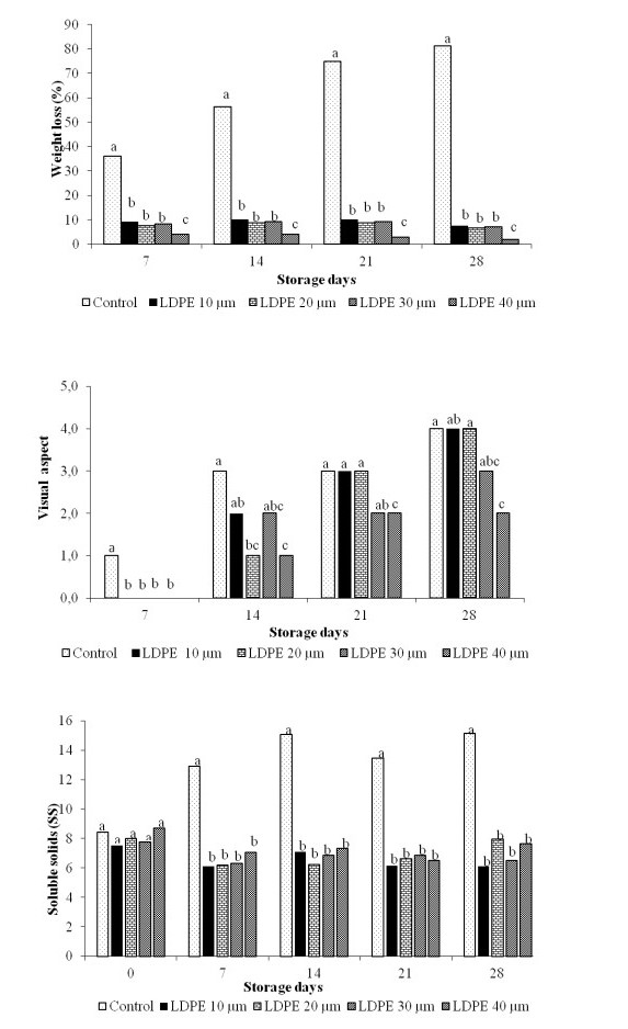
Okra (Abelmoschus esculentus L. Moench) is a vegetable crop of high nutritional value, which presents great losses after harvest when stored under poor storage conditions. The objective of this research was to evaluate the effect of different low-density polyethylene (LDPE) thicknesses on the preservation and post-harvest quality of okra fruits under different storage periods. The experiment was conducted in a completely randomized design, with nine replicates, in a 5 × 5 factorial scheme, corresponding to five forms of packaging at a temperature of 10 ± 1 ℃: no film and four LDPE thicknesses (10, 20, 30, and 40 µm) with five storage periods (0, 7, 14, 21, and 28 days). It was revealed that the use of LDPE plastic films provided lower loss of mass, higher fruit firmness containment of increase in soluble solids, and lower color change at 21 days of storage compared to no film. The LDPE thickness of 30 µm showed lower incidence of rotting, better appearance throughout storage, lower color changes, containment of increase in soluble solids content, higher chlorophyll, ascorbic acid, and total phenolic content compared to other forms of packaging, and is the most appropriate package for storing okra fruits up to 21 days, under refrigeration condition. The results of this study show that the thickness of LDPE has significant effects on the conservation and quality of okra. Our findings can be used to minimize post-harvest losses of okra during marketing.
Citation: Dalva Paulus, Sintieli Borges Ferreira, Dislaine Becker. Preservation and post-harvest quality of okra using low density polyethylene[J]. AIMS Agriculture and Food, 2021, 6(1): 321-336. doi: 10.3934/agrfood.2021020
Okra (Abelmoschus esculentus L. Moench) is a vegetable crop of high nutritional value, which presents great losses after harvest when stored under poor storage conditions. The objective of this research was to evaluate the effect of different low-density polyethylene (LDPE) thicknesses on the preservation and post-harvest quality of okra fruits under different storage periods. The experiment was conducted in a completely randomized design, with nine replicates, in a 5 × 5 factorial scheme, corresponding to five forms of packaging at a temperature of 10 ± 1 ℃: no film and four LDPE thicknesses (10, 20, 30, and 40 µm) with five storage periods (0, 7, 14, 21, and 28 days). It was revealed that the use of LDPE plastic films provided lower loss of mass, higher fruit firmness containment of increase in soluble solids, and lower color change at 21 days of storage compared to no film. The LDPE thickness of 30 µm showed lower incidence of rotting, better appearance throughout storage, lower color changes, containment of increase in soluble solids content, higher chlorophyll, ascorbic acid, and total phenolic content compared to other forms of packaging, and is the most appropriate package for storing okra fruits up to 21 days, under refrigeration condition. The results of this study show that the thickness of LDPE has significant effects on the conservation and quality of okra. Our findings can be used to minimize post-harvest losses of okra during marketing.

| [1] |
Kyriakopoulou OG, Arens P, Pelgrom KTB, et al. (2014) Genetic and morphological diversity of okra (Abelmoschus esculentus L. Moench.) genotypes and their possible relationships, with particular reference to Greek landraces. Sci Hortic 171: 58-70. doi: 10.1016/j.scienta.2014.03.029

|
| [2] |
Kumar S, Parekh MJ, Fougat RS, et al. (2017) Assessment of genetic diversity among okra genotypes using SSR markers. J Plant Biochem Biotechnol 26: 172-178. doi: 10.1007/s13562-016-0378-2
|
| [3] |
Petropoulos S, Fernandes Â, Barros L, et al. (2018) Chemical composition, nutritional value and antioxidant properties of Mediterranean okra genotypes in relation to harvest stage. Food Chem 242: 466-474. doi: 10.1016/j.foodchem.2017.09.082
|
| [4] |
Mota WF, Finger FL, Cecon PR, et al. (2010) Preservation and postharvest quality of okra under different temperatures and forms of storage. Hortic Bras 28: 12-18. doi: 10.1590/S0102-05362010000100003
|
| [5] |
Finger FL, Della-Justina ME, Casali VWD, et al. (2008) Temperature and modified atmosphere affect the quality of okra. Sci Agric 65: 360-364. doi: 10.1590/S0103-90162008000400006
|
| [6] |
Rani M, Singh J, Kumar D (2015) Effect of different packaging material on chlorophyll and ascorbic acid content of the okra. South Asian J Food Technol Environ 1: 86-88. doi: 10.46370/sajfte.2015.v01i01.12
|
| [7] | Mantilla SPS, Mano SB, Vital HC, et al. (2010) Modified atmosphere in food preservation. Acad J Agric Environ Sci 8: 437-448. |
| [8] |
Alvares CA, Stape JL, Sentelhas PC, et al. (2013) Köppen's climate classification map for Brazil. Meteorol Z 22: 711-728. doi: 10.1127/0941-2948/2013/0507
|
| [9] | Chitarra MIF, Chitarra AB (2005) Postharvest of fruits and vegetables: physiology and handling. Lavras: FAEPE, 785. |
| [10] |
Arnon DI (1949) Copper enzyme in isolated chloroplasts polyphenoloxidase in Beta vulgaris. Plant Physiol 24: 1-15. doi: 10.1104/pp.24.1.1
|
| [11] | Instituto AL (2008) Physico-chemical methods for food analysis. 4 Eds., Sã o Paulo: Intituto Adolfo Lutz, 1020. |
| [12] |
Singleton VL, Orthofer R, Lamuela-Raventors RM (1999) Analysis of total phenols and other oxidation substrates and antioxidants by means of Folin-Ciocalteu reagent. Methods in Enzymol 299: 152-178. doi: 10.1016/S0076-6879(99)99017-1
|
| [13] | Statistical Analysis System. SAS Studio (2017) Available from: http://www.sas.com/en_us/software/university-edition.html//. |
| [14] |
Sanches J, Valentini SRT, Benato E, et al. (2011) Modified atmosphere and refrigeration for the postharvest conservation of 'Fukuhara' loquat. Bragantia 70: 455-459. doi: 10.1590/S0006-87052011000200029
|
| [15] | Babarinde GO, Fabunmi OA (2009) Effects of packaging materials and storage temperature on quality of fresh okra (Abelmoschus esculentus) fruit. Agric Trop Subtrop 42: 151- 156. |
| [16] |
Singh S, Chaurasia SNS, Prasad I, et al. (2020) Nutritional quality and shelf life extension of capsicum (Capsicum annum) in expanded polyethylene biopolymer. Asian J Dairy Food Res 39: 40-48. doi: 10.18805/ajdfr.DR-1506
|
| [17] | Sanches J, Antoniali S, Passos FA (2012) Use of modified atmosphere in the post-harvest conservation of okra. Hortic Bras 30: 65-72. |
| [18] | Kader AA (2002) Postharvest technology of horticultural crops. Oakland: University of California, Agriculture and Natural Resources, 535. |
| [19] | Silva JS, Finger FL, Corrêa PC (2000) Fruit and vegetable storage. In: Silva JS (Ed.). Drying and Storage of Agricultural Products. Viçosa: Editora Aprenda Fácil, 469-502. |
| [20] |
Rupollo G, Gutkoski C, Martins IR, et al. (2006) Effect of humidity and hermetic storage period on natural contamination by fungi and production of mycotoxins in oat grains. Ciência e Agrotecnologia 30: 118-125. doi: 10.1590/S1413-70542006000100017
|
| [21] | Sanches J, Cia P, Antoniali S, et al. (2009) Quality of minimally processed broccoli from organic and conventional cultivation. Hortic Bras 27: 830-837. |
| [22] |
Santos AF, Silva SM, Alves RE (2006) Storage of Suriname cherry under modified atmosphere and refrigeration: I-postharvest chemical changes. Rev Bras Frutic 28: 36-41. doi: 10.1590/S0100-29452006000100013
|
| [23] |
Moretti CL, Pineli LLO (2005) Chemical and physical quality of eggplant fruits submitted to different postharvest treatments. Food Sci Technol 25: 339-344. doi: 10.1590/S0101-20612005000200027
|
| [24] | Mahajan BV, Dhillon WS, Siddhu MK, et al. (2016) Effect of packaging and storage environments on quality and shelf life of bell pepper (Capsicum annum L.). Indian J Agric Res Sci 86: 738-742. |
| [25] | Nascimento IB, Ferreira LE, Medeiros JF, et al. (2013) Post-harvest quality of okra submitted to different saline water laminas. Agropecuária Científica no Semiárido 9: 88-93. |
| [26] |
Dhall RK, Sharma SR, Mahajan BVC (2012) Development of post-harvest protocol of okra for export marketing. J Food Sci Technol 51: 1622-1625. doi: 10.1007/s13197-012-0669-0
|
| [27] |
Saberi B, Golding JB, Marques JR, et al. (2018) Application of biocomposite edible coatings based on pea starch and guar gum on quality, storability and shelf life of 'Valencia'oranges. Postharvest Biologyand Technol 137: 9-20. doi: 10.1016/j.postharvbio.2017.11.003
|
| [28] |
Chauhan OP, Nanjappa C, Ashok N, et al. (2015) Shellac and aloevera gel based surface coating for shelf life extension of tomatoes. J Food Sci Technol 52: 1200-1205. doi: 10.1007/s13197-013-1035-6
|
| [29] | Arango ZTM, Rodríguez MC, Campuzano OIM (2010) Frutos de uchuva (Physalis peruviana L.) ecotipo 'Colombia' mínimamente procesados, adicionados con microorganismos probióticos utilizando la ingeniería de matrices. Rev Fac Nac Agron Medellin 63: 5395-5407. |
| [30] | Costa AS, Ribeiro LR, Koblitz MGB (2011).Use of controlled and modified atmosphere in climacteric and non-climacteric fruits. Biol Sci Sitientibus Ser 11: 1-7. |
| [31] |
Gong Y, Mattheis JP (2003) Effect of ethylene and 1-methylclopropene on chlorophyll catabolism of broccoli florets. Plant Growth Regul 40: 33-38. doi: 10.1023/A:1023058003002
|
| [32] |
Hörtensteiner S (2013) Update on the biochemistry of chlorophyll breakdown. Plant Mol Biol 82: 505-517. doi: 10.1007/s11103-012-9940-z
|
| [33] |
Plaza L, Sanchez-Moreno C, Elez-Martinez P, et al. (2006) Effect of refrigerated storage on Vitamin C and antioxidant activity of orange juice processed by high pressure or pulsed electric fields with regard to low pasteurization. Eur Food Res Technol 223: 487-493. doi: 10.1007/s00217-005-0228-2
|
| [34] | Manas D, Bandopadhyay PK, Chakravarty A, et al. (2013) Changes in some biochemical characteristics in response to foliar applications of chelator and micronutrients in green pungent pepper. Int J Plant Physiol, Biochem 5: 25-35. |
| [35] |
Howard LR, Talcott ST, Brenes CH, et al. (2000) Changes in phytochemical and antioxidant activity of selected pepper cultivars (Capsicum sp.) as influenced by maturity. J Agric Food Chem 48: 1713-1720. doi: 10.1021/jf990916t
|
| [36] | Martins S, Mussatto S, Martinez Avila G, et al. (2011) Bioactive phenolic compounds: Production and extraction by solid-state fermentation. A review. Biotechnol Adv 29: 365-373. |
| [37] | Marinova D, Ribarova F, Atanassova M (2005) Total phenolics and flavonoids in Bulgarian fruits and vegetables. J Chem Technol Metall 40: 255-260. |
| [38] |
Sreeramulu D, Raghunath M (2010) Antioxidant activity and phenolic content of roots, tubers and vegetables commonly consumed in India. Food Res Int 43: 1017-1020. doi: 10.1016/j.foodres.2010.01.009
|
Figures(1) / Tables(6)

Dalva Paulus, Sintieli Borges Ferreira, Dislaine Becker. Preservation and post-harvest quality of okra using low density polyethylene[J]. AIMS Agriculture and Food, 2021, 6(1): 321-336. doi: 10.3934/agrfood.2021020


 DownLoad: