Citation: Sidra Abid Syed, Munaf Rashid, Samreen Hussain. Meta-analysis of voice disorders databases and applied machine learning techniques[J]. Mathematical Biosciences and Engineering, 2020, 17(6): 7958-7979. doi: 10.3934/mbe.2020404

| [1] |
S. Misono, S. Marmor, N. Roy, T. Mau, S. Cohen, Multi-institutional study of voice disorders and voice therapy referral, Otolaryngol. Head Neck Surgery, 155 (2016), 33-41. doi: 10.1177/0194599816639244

|
| [2] | P. Bradley, Voice disorders: Classification, Otolaryngol. Head Neck Surgery, (2010), 555-562. |
| [3] | M. Behlau, M. L. S. Dragone, L. Nagano, The voice that teaches: The teacher and oral communication in the classroom, 2004. |
| [4] | A. E. Aronson, Clinical voice disorders, 3 ed., INC. New York: Thieme Medical Publishers, 1990, p. 3-11. |
| [5] |
J. R. Spiegel, R. T. Sataloff, K. A. Emerich, The young adult voice, J. Voice, 11 (1997), 138-143. doi: 10.1016/S0892-1997(97)80069-0
|
| [6] | L. O. Ramig, K. Verdolini, Treatment efficacy: Voice disorders, J. Speech Lang. Hear. Res., 41 (1998), 101-106. |
| [7] |
J. Baker, The role of psychogenic and psychosocial factors in the development of functional voice disorders, J. Speech Lang. Pathol., 10 (2008), 210-230. doi: 10.1080/17549500701879661
|
| [8] | S. T. Kasama, A. G. Brasolotto, Vocal perception and life quality, Pro. Fono., 9 (2007), 19-28. |
| [9] |
L. P. Ferreira, J. G. Santos, M. F. B. Lima, Vocal sympton and its probable cause: Data colleting in a population, Rev. CEFAC, 11 (2009), 110-118. doi: 10.1590/S1516-18462009000100015
|
| [10] |
P. H. Dejonckere, P. Bradley, P. Clemente, G. Cornut G, L. C. Buchman, G. Friedrich, et al., A basic protocol for functional assessment of voice pathology, especially for investigating the efficacy of (phonosurgical) treatments and evaluating new assessment techniques, Eur. Arch. Otorhinolaryngol., 258 (2001), 77-82. doi: 10.1007/s004050000299
|
| [11] | U. Cesari, G. De Pietro, E. Marciano, C. Niri, G. Sannino, L. Verde, Voice disorder detection via an m-Health system: Design and results of a clinical study to evaluate Vox4Health, BioMed. Res. Int., 2018 (2018), 1-19. |
| [12] |
L. Verde, G. De Pietro, G. Sannino, Voice disorder identification by using machine learning techniques, IEEE Access, 6 (2018), 16246-16255. doi: 10.1109/ACCESS.2018.2816338
|
| [13] | A. G. David, J. B. Magnus, Diagnosing parkinson by using artificial neural networks and support vector machines, Global J. Comput. Sci. Technol., (2009), 63-71. |
| [14] | Saarbruecken Voice Database—Handbook, Stimmdatenbank.coli.uni-saarland.de. [Online]. Available: http://www.stimmdatenbank.coli.uni-saarland.de/help_en.php4. |
| [15] | M. OpenCourseWare, Lab Database | Laboratory on the Physiology, Acoustics, and Perception of Speech | Electrical Engineering and Computer Science | MIT OpenCourseWare, Ocw.mit.edu. [Online]. Available: https://ocw.mit.edu/courses/electrical-engineering-and-computer-science/6-542j-laboratory-on-the-physiology-acoustics-and-perception-of-speech-fall-2005/lab-database/ |
| [16] | K. Daoudi, B. Bertrac, On classification between normal and pathological voices using the MEEI-KayPENTAX database: Issues and consequences, INTERSPEECH-2014, Sep 2014, Singapour, Singapore. ffhal-01010857 |
| [17] | N. Sáenz-Lechón, J. I. Godino-Llorente, V. Osma-Ruiz, P. Gómez-Vilda, Methodological issues in the development of automatic systems for voice pathology detection, Biomed. Signal Process. Control, 1 (2006), 120-128. |
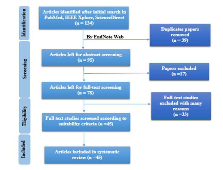
| [18] | A. Liberati, D. G. Altman, J. Tetzlaff, C. Mulrow, P. C. Gøtzsche, J. P. A. Ioannidis, et al., The PRISMA statement for reporting systematic reviews and meta-analyses of studies that evaluate healthcare interventions: Explanation and elaboration, BMJ, 339 (2009). |
| [19] | A. Al-Nasheri, G. Muhammad, M. Alsulaiman, Z. Ali, K. H. Malki, T. A. Mesallam, et al., Voice pathology detection and classification using auto-correlation and entropy features in different frequency regions, IEEE Access, 6, 6961-6974. |
| [20] | A. Al-Nasheri, G. Muhammad, M. Alsulaiman, Z. Ali, T. A. Mesallam, M. Farahat, et al., An investigation of multidimensional voice program parameters in three different databases for voice pathology detection and classification, J. Voice, 31 (2017), 113.e9-e18. |
| [21] |
A. Al-Nasheri, G. Muhammad, M. Alsulaiman, Z. Ali, Investigation of voice pathology detection and classification on different frequency regions using correlation functions, J. Voice, 31 (2017), 3-15. doi: 10.1016/j.jvoice.2016.01.014
|
| [22] | Z. Ali, M. Alsulaiman, G. Muhammad, I. Elamvazuthi, A. Al-Nasheri, T. A. Mesallam, K. H. Malki, et al., Intra- and inter-database study for Arabic, English, and German databases: Do conventional speech features detect voice pathology?, J. Voice, 31 (2017), 386.e1-e8. |
| [23] | E. S. Fonseca, R. C. Guido, S. B. Junior, H. Dezani, R. R. Gati, D. C. Mosconi Pereira, Acoustic investigation of speech pathologies based on the discriminative paraconsistent machine (DPM), Biomed. Signal Process. Control, 55 (2020). |
| [24] |
J. A. Gómez-García, L. Moro-Velázquez, J. Mendes-Laureano, G. Castellanos-Dominguez, J. I. Godino-Llorente, Emulating the perceptual capabilities of a human evaluator to map the GRB scale for the assessment of voice disorders, Eng. Appl. Artific. Intell., 82 (2019), 236--251. doi: 10.1016/j.engappai.2019.03.027
|
| [25] |
V. Guedes, F. Teixeira, A. Oliveira, J. Fernandes, L. Silva, A. Junior, et al., Transfer Learning with AudioSet to Voice Pathologies Identification in Continuous Speech, Proced. Comput. Sci., 164 (2019), 662-669. doi: 10.1016/j.procs.2019.12.233
|
| [26] |
I. Hammami, L. Salhi, S. Labidi, Voice pathologies classification and detection using EMD- DWT analysis based on higher order statistic features, IRBM, 41 (2020), 161-171. doi: 10.1016/j.irbm.2019.11.004
|
| [27] |
D. Hemmerling, A. Skalski, J. Gajda, Voice data mining for laryngeal pathology assessment, Comput. Biol. Med., 69 (2016), 270-276. doi: 10.1016/j.compbiomed.2015.07.026
|
| [28] | J. Moon, S. Kim, An approach on a combination of higher-order statistics and higher-order differential energy operator for detecting pathological voice with machine learning, 2018 International Conference on Information and Communication Technology Convergence (ICTC), 17-19 Oct. 2018, pp. 46-51. |
| [29] | K. Ezzine, M. Frikha, Investigation of glottal flow parameters for voice pathology detection on SVD and MEEI databases, 2018 4th International Conference on Advanced Technologies for Signal and Image Processing (ATSIP), 21-24 March 2018, pp. 1-6. |
| [30] | M. Markaki, Y. Stylianou, Using modulation spectra for voice pathology detection and classification, 2009 Annual International Conference of the IEEE Engineering in Medicine and Biology Society, 3-6 Sept. 2009, pp. 2514-2517. |
| [31] |
M. Markaki, Y. Stylianou, Voice pathology detection and discrimination based on modulation spectral features, IEEE Transact. Aud. Speech Langu. Process, 19 (2011), 1938-1948. doi: 10.1109/TASL.2010.2104141
|
| [32] | J. M. Miramont, J. F. Restrepo, J. Codino, C. Jackson-Menaldi, G. Schlotthauer, Voice signal typing using a pattern recognition approach, J. Voice, 2020. |
| [33] |
G. Muhammad, M. Alsulaiman, Z. Ali, T. A. Mesallam, M. Farahat, K. H. Malki, et al., Voice pathology detection using interlaced derivative pattern on glottal source excitation, Biomed. Signal Process. Control, 31 (2017), 156-164. doi: 10.1016/j.bspc.2016.08.002
|
| [34] | S. E. Shia, T. Jayasree, Detection of pathological voices using discrete wavelet transform and artificial neural networks, 2017 IEEE International Conference on Intelligent Techniques in Control, Optimization and Signal Processing (INCOS), 23-25 March 2017, pp. 1-6. |
| [35] |
S. R. Kadiri, P. Alku, Analysis and detection of pathological voice using glottal source features, IEEE J. Select. Topics Signal Process., 14 (2020), 367-379. doi: 10.1109/JSTSP.2019.2957988
|
| [36] |
T. Zhang, Y. Shao, Y. Wu, Z. Pang, G. Liu, Multiple vowels repair based on pitch extraction and line spectrum pair feature for voice disorder, IEEE J. Biomed. Health Inform., 24 (2020), 1940-1951. doi: 10.1109/JBHI.2020.2978103
|
| [37] |
F. Teixeira, J. Fernandes, V. Guedes, A. Junior, J. P. Teixeira, Classification of control/pathologic subjects with support vector machines, Proced. Comput. Sci., 138 (2018), 272-279. doi: 10.1016/j.procs.2018.10.039
|
| [38] |
J. P. Teixeira, P. O. Fernandes, N. Alves, Vocal acoustic analysis—classification of dysphonic voices with artificial neural networks, Proced. Comput. Sci., 121 (2017), 19-26. doi: 10.1016/j.procs.2017.11.004
|
| [39] |
G. Muhammad, M. Melhem, Pathological voice detection and binary classification using MPEG-7 audio features, Biomed. Signal Process. Control, 11 (2014), 1-9. doi: 10.1016/j.bspc.2014.02.001
|
| [40] |
J. Nayak, P. S. Bhat, R. Acharya, U. V. Aithal, Classification and analysis of speech abnormalities, ITBM-RBM, 26 (2005), 319-327. doi: 10.1016/j.rbmret.2005.05.002
|
| [41] | Z. Ali, I. Elamvazuthi, M. Alsulaiman, G. Muhammad, Automatic voice pathology detection with running speech by using estimation of auditory spectrum and cepstral coefficients based on the all-pole model, J. Voice, 30 (2016), 757.e7-e19. |
| [42] |
R. Amami, A. Smiti, An incremental method combining density clustering and support vector machines for voice pathology detection, Comput. Electr. Eng., 57 (2017), 257-265. doi: 10.1016/j.compeleceng.2016.08.021
|
| [43] | J. D. Arias-Londoño, J. I. Godino-Llorente, N. Sáenz-Lechón, V. Osma-Ruiz, G. Castellanos- Domínguez, An improved method for voice pathology detection by means of a HMM-based feature space transformation, Patt. Recogn., 43 (2010), 3100-3112. |
| [44] |
M. K. Arjmandi, M. Pooyan, M. Mikaili, M. Vali, A. Moqarehzadeh, Identification of voice disorders using long-time features and support vector machine with different feature reduction methods, J. Voice, 25 (2011), e275-e289. doi: 10.1016/j.jvoice.2010.08.003
|
| [45] |
R. R. A. Barreira, L. L. Ling, Kullback-leibler divergence and sample skewness for pathological voice quality assessment, Biomed. Signal Process. Control, 57 (2020), 101697. doi: 10.1016/j.bspc.2019.101697
|
| [46] | C. R. Francis, V. V. Nair, S. Radhika, A scale invariant technique for detection of voice disorders using Modified Mellin Transform, 2016 International Conference on Emerging Technological Trends (ICETT), 21-22 Oct. 2016, pp. 1-6. |
| [47] | H. Cordeiro, J. Fonseca, I. Guimarães, C. Meneses, Hierarchical classification and system combination for automatically identifying physiological and neuromuscular laryngeal pathologies, J. Voice, 31 (2017), 384. |
| [48] |
H. T. Cordeiro, C. M. Ribeiro, Spectral envelope first peak and periodic component in pathological voices: A spectral analysis, Proced. Comput. Sci., 138 (2018), 64-71. doi: 10.1016/j.procs.2018.10.010
|
| [49] |
S. H. Fang, Y. Tsao, M. J. Hsiao, J. Y. Chen, Y. H. Lai, F. C. Lin, et al., Detection of pathological voice using cepstrum vectors: A deep learning approach, J. Voice, 33 (2019), 634-641. doi: 10.1016/j.jvoice.2018.02.003
|
| [50] | G. Muhammad, Voice pathology detection using vocal tract area, 2013 European Modelling Symposium, 20-22 Nov. 2013, pp. 164-168. |
| [51] |
H. Ghasemzadeh, M. Tajik Khass, M. Khalil Arjmandi, M. Pooyan, Detection of vocal disorders based on phase space parameters and Lyapunov spectrum, Biomed. Signal Process. Control, 22 (2015), 135-145. doi: 10.1016/j.bspc.2015.07.002
|
| [52] | J. I. Godino-Llorente, R. Fraile, N. Sáenz-Lechón, V. Osma-Ruiz, P. Gómez-Vilda, Automatic detection of voice impairments from text-dependent running speech, Biomed. Signal Process. Control, 4 (2009), 176-182. |
| [53] |
M. Hariharan, K. Polat, R. Sindhu, S. Yaacob, A hybrid expert system approach for telemonitoring of vocal fold pathology, Appl. Soft Comput., 13 (2013), 4148-4161. doi: 10.1016/j.asoc.2013.06.004
|
| [54] |
A. Mahmood, A solution to the security authentication problem in smart houses based on speech, Proced. Comput. Sci., 155 (2019), 606-611. doi: 10.1016/j.procs.2019.08.085
|
| [55] |
J. Mekyska, E. Janousova, P. Gomez-Vilda, Z. Smekal, I. Rektorova, I. Eliasova, et al., Robust and complex approach of pathological speech signal analysis, Neurocomputing, 167 (2015), 94-111. doi: 10.1016/j.neucom.2015.02.085
|
| [56] |
G. Muhammad, M. Melhem, Pathological voice detection and binary classification using MPEG-7 audio features, Biomed. Signal Process. Control, 11 (2014), 1-9. doi: 10.1016/j.bspc.2014.02.001
|
| [57] |
J. Nayak, P. S. Bhat, R. Acharya, U. V. Aithal, Classification and analysis of speech abnormalities, ITBM-RBM, 26 (2005), 319-327. doi: 10.1016/j.rbmret.2005.05.002
|
| [58] | P. Henriquez, J. B. Alonso, M. A. Ferrer, C. M. Travieso, J. I. Godino-Llorente, F. Diaz-de- Maria, Characterization of healthy and pathological voice through measures based on nonlinear dynamics, IEEE Transact. Audio Speech Lang. Process., 17 (2009), 1186-1195. |
| [59] | P. Salehi, Using patient's speech signal for vocal ford disorders detection based on lifting scheme, in 2015 2nd International Conference on Knowledge-Based Engineering and Innovation (KBEI), 5-6 Nov. 2015, pp. 561-568. |
| [60] | N. Sáenz-Lechón, J. I. Godino-Llorente, V. Osma-Ruiz, P. Gómez-Vilda, Methodological issues in the development of automatic systems for voice pathology detection, Biomed. Signal Process. Control, 1 (2006), 120-128. |
| [61] | C. M. Travieso, J. B. Alonso, J. R. Orozco-Arroyave, J. F. Vargas-Bonilla, E. Nöth, A. G. Ravelo- García, Detection of different voice diseases based on the nonlinear characterization of speech signals, Expert Systems Appl., 82 (2017), 184-195. |
| [62] | T. A. Mesallam, F. Mohamed, K. H. Malki, A. Mansour, A. Zulfiqar, A. N. Ahmed, et al., Development of the arabic voice pathology database and its evaluation by using speech features and machine learning algorithms, J. Healthc. Eng., (2017), 1-13. |
| [63] | K. Uma Rani, Mallikarjun S Holi, A comparative study of neural networks and support vector machines for neurological disordered voice classification, Inter. J. Eng. Res. Techol., 3 (2014). |
| [64] | J. Godino-Llorente, P. Gómez-Vilda, N. Sáenz-Lechón, M. Blanco-Velasco, F. Cruz-Roldán, M. Ferrer-Ballester, Support vector machines applied to the detection of voice disorders, Nonlin. Analy. Algor. Speech Process., (2006), 219-230. |
| [65] | S. Huang, N. Cai, P. P. Pacheco, S. Narrandes, Y. Wang, W. Xu, Applications of support vector machine (svm) learning in cancer genomics, Cancer Genom. Proteom., 15 (2018). |
| [66] |
S. Yue, P. Li, P. Hao, SVM classification: Its contents and challenges, Appl. Math. J. Chinese Univer., 18 (2003), 332-342. doi: 10.1007/s11766-003-0059-5
|
| [67] | D. Reynolds, Gaussian Mixture Models, In: S. Z. Li, A. Jain (eds), Encyclopedia of Biometrics, Springer, Boston, MA, 2009. |
| [68] | L. Breiman, J. Friedman, C. J. Stone, R. A. Olshen, Classification and regression trees, Boca Raton, FL: CRC press, 1984. |
| [69] | L. Breiman, Bagging predictors, Mach. Learn., 24 (1996), 123-140. |
| [70] |
S. Indolia, A. Goswami, S. Mishra, P. Asopa, Conceptual understanding of convolutional neural network- A deep learning approach, Proced. Computer Sci., 132 (2018), 679-688. doi: 10.1016/j.procs.2018.05.069
|
| [71] |
R. Yamashita, M. Nishio, R. Do, K. Togashi, Convolutional neural networks: An overview and application in radiology, Insights Imag., 9 (2018), 611-629. doi: 10.1007/s13244-018-0639-9
|
| [72] |
V. Parsa, D. G. Jamieson, Identification of pathological voices using glottal noise measures, J. Speech Langu. Hear. Res., 43 (2000), 469-485. doi: 10.1044/jslhr.4302.469
|
| [73] |
D. D. Deliyski, H. S. Shaw, M. K. Evans, Influence of sampling rate on accuracy and reliability of acoustic voice analysis, Logoped. Phoniatr. Vocol., 30 (2005), 55-62. doi: 10.1080/1401543051006721
|
| [74] |
Y. Horii, Jitter and shimmer in sustained vocal fry phonation, Folia Phoniatr., 37 (1985), 81-86. doi: 10.1159/000265785
|
| [75] |
J. L. Fitch, Consistency of fundamental frequency and perturbation in repeated phonations of sustained vowels, reading, and connected speech, J. Speech Hear. Disord., 55 (1990), 360-363. doi: 10.1044/jshd.5502.360
|
| [76] | T. Mesallam, M. Farahat, K. Malki, M. Alsulaiman, Z. Ali, A. Al-nasheri, et al., Development of the arabic voice pathology database and its evaluation by using speech features and machine learning algorithms, J. Healthc. Eng., 2017, 1-13. |
| [77] | P. Harar, Z. Galaz, J. Alonso-Hernandez, J. Mekyska, R. Burget, Z. Smekal, Towards robust voice pathology detection, Neural Comput. Appl., 2018. |
| [78] |
D. D. Mehta, R. E. Hillman, Voice assessment: Updates on perceptual, acoustic, aerodynamic, and endoscopic imaging methods, Curr. Opin. Otolaryngol. Head Neck Surg., 16 (2008), 211. doi: 10.1097/MOO.0b013e3282fe96ce
|
Figures(9) / Tables(2)

Sidra Abid Syed, Munaf Rashid, Samreen Hussain. Meta-analysis of voice disorders databases and applied machine learning techniques[J]. Mathematical Biosciences and Engineering, 2020, 17(6): 7958-7979. doi: 10.3934/mbe.2020404


 DownLoad: