Integrating LSTM with Fama-French six factor model for predicting portfolio returns: Evidence from Shenzhen stock market China

Tahir Afzal; Muhammad Asim Afridi; Muhammad Naveed Jan; Tahir Afzal; Muhammad Asim Afridi; Muhammad Naveed Jan

doi:10.3934/DSFE.2025009

Data Science in Finance and Economics

2025, Volume 5, Issue 2: 177-204. doi: 10.3934/DSFE.2025009

Previous Article Next Article

Research article

Integrating LSTM with Fama-French six factor model for predicting portfolio returns: Evidence from Shenzhen stock market China

1.
Department of Management Sciences, COMSATS University Islamabad, Abbottabad Campus, Abbottabad 22060, Pakistan
2.
Department of Economics, COMSATS University Islamabad, Abbottabad Campus, Abbottabad 22060, Pakistan

Received: 04 November 2024 Revised: 29 March 2025 Accepted: 18 April 2025 Published: 19 May 2025
JEL Codes: G11, G12, G17, C8

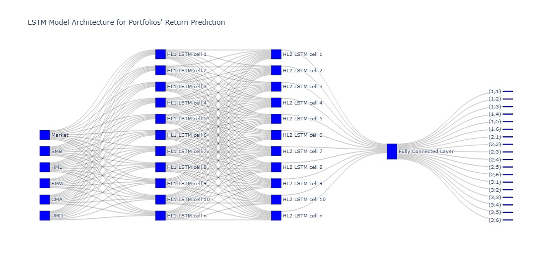
The study aimed to examine the effectiveness of long short-term memory (LSTM) model in predicting portfolio returns employing Fama and French's six-factor model. Monthly data were collected for A-share prices for firms listed on the Shenzhen Stock Exchange, China, for the period extended over 25 years (1997–2022). Portfolios are constructed on bivariate dependent sorting using the beta and downside beta. The random forest model was employed as a surrogate for LSTM to detect the nonlinear and threshold-based conditional relationship between risk factors and portfolio returns. The findings of the study reveal that LSTM has robust predictive ability and effectively captures the relationship between risk factors and portfolio returns. The relationship is more conspicuous in high downside risk portfolios than in the medium and high beta portfolio groups. Furthermore, portfolios within the high beta group, regardless of their downside beta levels, exhibit positive returns. The study suggests that investors need to consider high-risk portfolios for stable earnings and predictive returns.

Keywords:

Citation: Tahir Afzal, Muhammad Asim Afridi, Muhammad Naveed Jan. Integrating LSTM with Fama-French six factor model for predicting portfolio returns: Evidence from Shenzhen stock market China[J]. Data Science in Finance and Economics, 2025, 5(2): 177-204. doi: 10.3934/DSFE.2025009

Related Papers:

[1]	Yuhong Huo, Gourav Mandal, Lakshmi Narayan Guin, Santabrata Chakravarty, Renji Han . Allee effect-driven complexity in a spatiotemporal predator-prey system with fear factor. Mathematical Biosciences and Engineering, 2023, 20(10): 18820-18860. doi: 10.3934/mbe.2023834
[2]	Yue Xing, Weihua Jiang, Xun Cao . Multi-stable and spatiotemporal staggered patterns in a predator-prey model with predator-taxis and delay. Mathematical Biosciences and Engineering, 2023, 20(10): 18413-18444. doi: 10.3934/mbe.2023818
[3]	Yongli Cai, Malay Banerjee, Yun Kang, Weiming Wang . Spatiotemporal complexity in a predator--prey model with weak Allee effects. Mathematical Biosciences and Engineering, 2014, 11(6): 1247-1274. doi: 10.3934/mbe.2014.11.1247
[4]	Fang Liu, Yanfei Du . Spatiotemporal dynamics of a diffusive predator-prey model with delay and Allee effect in predator. Mathematical Biosciences and Engineering, 2023, 20(11): 19372-19400. doi: 10.3934/mbe.2023857
[5]	Ranjit Kumar Upadhyay, Swati Mishra . Population dynamic consequences of fearful prey in a spatiotemporal predator-prey system. Mathematical Biosciences and Engineering, 2019, 16(1): 338-372. doi: 10.3934/mbe.2019017
[6]	Sangeeta Kumari, Sidharth Menon, Abhirami K . Dynamical system of quokka population depicting Fennecaphobia by Vulpes vulpes. Mathematical Biosciences and Engineering, 2025, 22(6): 1342-1363. doi: 10.3934/mbe.2025050
[7]	Meiling Zhu, Huijun Xu . Dynamics of a delayed reaction-diffusion predator-prey model with the effect of the toxins. Mathematical Biosciences and Engineering, 2023, 20(4): 6894-6911. doi: 10.3934/mbe.2023297
[8]	Tingting Ma, Xinzhu Meng . Global analysis and Hopf-bifurcation in a cross-diffusion prey-predator system with fear effect and predator cannibalism. Mathematical Biosciences and Engineering, 2022, 19(6): 6040-6071. doi: 10.3934/mbe.2022282
[9]	Guangxun Sun, Binxiang Dai . Stability and bifurcation of a delayed diffusive predator-prey system with food-limited and nonlinear harvesting. Mathematical Biosciences and Engineering, 2020, 17(4): 3520-3552. doi: 10.3934/mbe.2020199
[10]	Swadesh Pal, Malay Banerjee, Vitaly Volpert . Spatio-temporal Bazykin’s model with space-time nonlocality. Mathematical Biosciences and Engineering, 2020, 17(5): 4801-4824. doi: 10.3934/mbe.2020262

Abstract

References

[1]	Agarwal PK, Pradhan HK (2018) Mutual fund performance using unconditional multifactor models: Evidence from India. J Emerg Mark Financ 17: 157–184. https://doi.org/10.1177/0972652718777056 doi: 10.1177/0972652718777056
[2]	Aharoni G, Grundy B, Zeng Q (2013). Stock returns and the Miller Modigliani valuation formula: Revisiting the Fama French analysis. J Financ Econ 110: 347–357. https://doi.org/10.1016/j.jfineco.2013.08.003 doi: 10.1016/j.jfineco.2013.08.003
[3]	Aminimehr A, Raoofi A, Aminimehr A, et al. (2022) A comprehensive study of market prediction from efficient market hypothesis up to late intelligent market prediction approaches. Comput Econ 60: 781–815. https://doi.org/10.1007/s10614-022-10283-1 doi: 10.1007/s10614-022-10283-1
[4]	Ang A, Chen JS, Xing Y (2002) Downside correlation and expected stock returns. EFA 2002 Berlin Meetings. https://doi.org/10.2139/ssrn.282986
[5]	Ashwood AJ (2013) Portfolio selection using artificial intelligence, Queensland University of Technology. Available from: https://eprints.qut.edu.au/66229/1/Andrew_Ashwood_Thesis.pdf.
[6]	Ayub U, Kausar S, Noreen U, et al. (2020) Downside risk-based six-factor capital asset pricing model (CAPM): A new paradigm in asset pricing. Sustainability 12: 6756. https://doi.org/10.3390/SU12176756 doi: 10.3390/SU12176756
[7]	Bhandari HN, Rimal B, Pokhrel NR, et al. (2022) Predicting stock market index using LSTM. Mach Learn Appl 9: 100320. https://doi.org/10.1016/j.mlwa.2022.100320 doi: 10.1016/j.mlwa.2022.100320
[8]	Buditomo B, Candra S, Soetanto TV (2024) Fama and french five-factor study of stock market in indonesia. Int J Organ Behav Policy 3: 39–52. https://doi.org/10.9744/ijobp.3.1.39-52 doi: 10.9744/ijobp.3.1.39-52
[9]	Carhart MM (1997) On persistence in mutual fund performance. J Financ 52: 57–82. https://doi.org/10.1111/j.1540-6261.1997.tb03808.x doi: 10.1111/j.1540-6261.1997.tb03808.x
[10]	Carpenter JN, Whitelaw RF (2017) The development of China's stock market and stakes for the global economy. Ann Rev Financ Econ 9: 233–257. https://doi.org/10.1146/annurev-financial-110716-032333 doi: 10.1146/annurev-financial-110716-032333
[11]	Cederburg S, O'Doherty MS (2015) Asset-pricing anomalies at the firm level. J Econ 186: 113–128. https://doi.org/https://doi.org/10.1016/j.jeconom.2014.06.004 doi: 10.1016/j.jeconom.2014.06.004
[12]	Daniel K, Moskowitz TJ (2014) Momentum crashes. NATIONAL BUREAU OF ECONOMIC RESEARCH. Available from: http://www.nber.org/papers/w20439.
[13]	Diallo B, Bagudu A, Zhang Q (2023) Fama–French three versus five, which model is better? A machine learning approach. J Forecast 42: 1461–1475. https://doi.org/https://doi.org/10.1002/for.2970 doi: 10.1002/for.2970
[14]	Dirkx P, Peter FJ (2020) The Fama-French five-factor model plus momentum: Evidence for the german market. Schmalenbach Bus Rev 72: 661–684. https://doi.org/10.1007/s41464-020-00105-y doi: 10.1007/s41464-020-00105-y
[15]	Estrada J (2007) Mean-semivariance behavior: Downside risk and capital asset pricing. Int Rev Econ Financ 16: 169–185. https://doi.org/10.1016/j.iref.2005.03.003 doi: 10.1016/j.iref.2005.03.003
[16]	Estrada J, Serra AP (2005) Risk and return in emerging markets: Family matters. J Multinational Financ Manag 15: 257–272. https://doi.org/10.1016/j.mulfin.2004.09.002 doi: 10.1016/j.mulfin.2004.09.002
[17]	Fama EF, French KR (1992) The cross‐section of expected stock returns. J Financ 47: 427–465. https://doi.org/10.1111/j.1540-6261.1992.tb04398.x doi: 10.1111/j.1540-6261.1992.tb04398.x
[18]	Fama EF, French KR (2006) Profitability, investment and average returns. J Financ Econ 82: 491–518. https://doi.org/10.1016/j.jfineco.2005.09.009 doi: 10.1016/j.jfineco.2005.09.009
[19]	Fama EF, French KR (2015) A five-factor asset pricing model. J Financ Econ 116: 1–22. https://doi.org/10.1016/j.jfineco.2014.10.010 doi: 10.1016/j.jfineco.2014.10.010
[20]	Fama EF, French KR (2018) Choosing factors. J Financ Econ 128: 234–252. https://doi.org/10.1016/j.jfineco.2018.02.012 doi: 10.1016/j.jfineco.2018.02.012
[21]	Feng G, He J, Polson NG (2018) Deep learning for predicting asset returns. arXiv Preprint 1804: 1–23.
[22]	Feng Z, Runtong Z, Lingyun H (2007) A prospective study of the price behaviors of Chinese stock markets. Chinese Control Conference, 558–562.
[23]	Galagedera DU (2009) An analytical framework for explaining relative performance of CAPM beta and downside beta. Int J Theor Appl Financ 12: 341–358. https://doi.org/10.1142/S0219024909005257 doi: 10.1142/S0219024909005257
[24]	Giglio S, Kelly B, Xiu D (2022) Factor models, machine learning, and asset pricing. Ann Rev Financ Econ 14: 337–368. https://doi.org/10.1146/annurev-financial-101521-104735 doi: 10.1146/annurev-financial-101521-104735
[25]	Goo Y, Wang C (2024) Do there exist nonlinear phenomena of the Fama-French six factors on stock returns? An empirical investigation on the Taiwan stock market. Modern Econ 15: 394–412. https://doi.org/10.4236/me.2024.154021 doi: 10.4236/me.2024.154021
[26]	Hall P, Gill N (2019) An introduction to machine learning interpretability. O'Reilly Media, Incorporated.
[27]	Hochreiter S, Schmidhuber J (1997) Long short-term memory. Neural Compu 9: 1735–1780.
[28]	Hu GX, Chen C, Shao Y, et al. (2019) Fama–French in China: Size and Value factors in Chinese stock returns. Int Rev Financ 19: 3–44. https://doi.org/10.1111/irfi.12177 doi: 10.1111/irfi.12177
[29]	Hu GX, Pan J, Wang J (2018) Chinese capital market: An empirical overview. NBER WORKING PAPER SERIES. Available from: https://www.nber.org/system/files/working_papers/w24346/w24346.pdf.
[30]	Jegadeesh N, Titman S (1993) Returns to buying winners and selling losers: Implications for stock market efficiency. J Financ 48: 65–91. https://doi.org/10.2307/2328882 doi: 10.2307/2328882
[31]	Jia H (2023) Comparison on Asset Pricing Models: Application of CAPM, Fama-French 3 Factors model and Fama-French 5 factors model. BCP Bus Manag 40: 119–127. https://doi.org/10.54691/bcpbm.v40i.4367 doi: 10.54691/bcpbm.v40i.4367
[32]	Jinghan C (2010) Trading preference of Chinese investors and its impact on stock volatility. Rev Financ Stud 3: 53–64.
[33]	Joshi V (2024) Cross-section of expected stock returns: An application of Fama-French Five Factor Model in Nepal. Batuk 10: 72–89. https://doi.org/10.3126/batuk.v10i1.62299 doi: 10.3126/batuk.v10i1.62299
[34]	Kazmi M, Noreen U, Jadoon IA, et al. (2021) Downside beta and downside gamma: In search for a better capital asset pricing model. Risks 9: 223. https://doi.org/10.3390/risks9120223 doi: 10.3390/risks9120223
[35]	Kundlia S, Verma D (2021) Illiquidity premium in the Indian stock market: An empirical study. Asian Econ Financ Rev 11: 501–511. https://doi.org/10.18488/JOURNAL.AEFR.2021.116.501.511 doi: 10.18488/JOURNAL.AEFR.2021.116.501.511
[36]	Lintner J (1965) Security prices, risk, and maximal gains from diversification. J Financ 20: 587–615. https://doi.org/10.2307/2977249 doi: 10.2307/2977249
[37]	Liu J (2019) A novel downside risk measure and expected returns. The World Bank. https://doi.org/10.2139/ssrn.3406944 doi: 10.2139/ssrn.3406944
[38]	Liu X, Wang X (2023) Stock investment strategies with time-varying co-movements between energy market and global financial market. Highlights Busi Econ Manag 21: 862–866.
[39]	Markowitz H (1952) Portfolio selection. J Financ 7: 77–91.
[40]	Mahpudin E (2020) The Effect of Macroeconomics on Stock Price Index in the Republic of China. Int J Econ Bus Adm VIII: 228–236. https://doi.org/10.35808/ijeba/511
[41]	Miller MH, Modigliani F (1961) Dividend policy, growth, and the valuation of shares. J Bus 34: 411. https://doi.org/10.1086/294442 doi: 10.1086/294442
[42]	Miralles-Quirós JL, Miralles-Quirós MM, Nogueira JM (2020) Sustainable development goals and investment strategies: The profitability of using Five-Factor Fama-French alphas. Sustainability 12: 1–16. https://doi.org/10.3390/su12051842 doi: 10.3390/su12051842
[43]	Molnar C (2020) Interpretable machine learning. Lulu. com.
[44]	Mossin J (1966) Equilibrium in a capital asset market. Econometrica 34: 768–783. https://doi.org/10.2307/1910098 doi: 10.2307/1910098
[45]	Novy-Marx R (2013) The other side of value: The gross profitability premium. J Financ Econ 108: 1–28. https://doi.org/10.1016/j.jfineco.2013.01.003 doi: 10.1016/j.jfineco.2013.01.003
[46]	Petrozziello A, Troiano L, Serra A, et al. (2022) Deep learning for volatility forecasting in asset management. Soft Comput 26: 8553–8574. https://doi.org/10.1007/s00500-022-07161-1 doi: 10.1007/s00500-022-07161-1
[47]	Sharma K, Bhalla R (2022) Stock market prediction techniques: A review paper. Second International Conference on Sustainable Technologies for Computational Intelligence, 175–188. https://doi.org/10.1007/978-981-16-4641-6_15 doi: 10.1007/978-981-16-4641-6_15
[48]	Sharpe WF (1964) Capital asset prices: A theory of market equilibrium under conditions of risk. J Financ 19: 425–442. https://doi.org/10.1111/j.1540-6261.1964.tb02865.x doi: 10.1111/j.1540-6261.1964.tb02865.x
[49]	Sharpe WF (1966) Mutual fund performance. J Bus 39: 119–138. http://www.jstor.org/stable/2351741
[50]	Singh K, Singh A, Prakash P (2023) Testing factor models in an emerging market: Evidence from India. Int J Manag Financ 19: 203–232. https://doi.org/10.1108/IJMF-05-2021-0245 doi: 10.1108/IJMF-05-2021-0245
[51]	Sortino FA, Van Der Meer R (1991) Downside risk. J Portfolio Manag 17: 27.
[52]	Staudemeyer RC, Morris ER (2019) Understanding LSTM -- a tutorial into long short-term memory Recurrent Neural Networks. arXiv Preprint 1909: 09586. http://arXiv.org/abs/1909.09586
[53]	Sun J, Manger G (2012) Listing on the Shenzhen Stock Exchange: Behavioural finance implications. ASBBS Proc 19: 874–889. http://search.proquest.com/docview/1445142469?accountid = 79789
[54]	Tan L, Zhang X, Zhang X (2024) Retail and institutional investor trading behaviours: Evidence from China. Ann Rev Financ Econ 16: 459–483.
[55]	Yang P, Yang L (2022) Asset pricing and nominal price illusion in China. Humanit Soc Sci Communicat 9: 1–9. https://doi.org/10.1057/s41599-022-01133-4 doi: 10.1057/s41599-022-01133-4
[56]	Zaghouani CA, Mezzez HD (2020). Evidence on aggregate volatility risk premium for the French Stock Market. Managerial Financ 46: 72–91. https://doi.org/10.1108/MF-11-2018-0535 doi: 10.1108/MF-11-2018-0535
[57]	Zhang C (2022) Asset pricing and deep learning. arXiv Preprint 2209: 1–18. http://arXiv.org/abs/2209.12014
[58]	Zheng Y, Wen F, Deng H, et al. (2022) The relationship between carbon market attention and the EU CET market: Evidence from different market conditions. Financ Res Lett 50: 103140. https://doi.org/https://doi.org/10.1016/j.frl.2022.103140 doi: 10.1016/j.frl.2022.103140

DSFE-05-02-009-S001.pdf

This article has been cited by:

1.	Sourav Kumar Sasmal, Yasuhiro Takeuchi, Evolutionary dynamics of single species model with Allee effects and aposematism, 2021, 58, 14681218, 103233, 10.1016/j.nonrwa.2020.103233
2.	Sourav Kumar Sasmal, Balram Dubey, Diffusive patterns in a predator–prey system with fear and hunting cooperation, 2022, 137, 2190-5444, 10.1140/epjp/s13360-022-02497-x
3.	Sourav Kumar Sasmal, Yasuhiro Takeuchi, Editorial: Mathematical Modeling to Solve the Problems in Life Sciences, 2020, 17, 1551-0018, 2967, 10.3934/mbe.2020167
4.	Balram Dubey, Sourav Kumar Sasmal, Anand Sudarshan, Consequences of fear effect and prey refuge on the Turing patterns in a delayed predator–prey system, 2022, 32, 1054-1500, 123132, 10.1063/5.0126782
5.	Balram Dubey, Study of a cannibalistic prey–predator model with Allee effect in prey under the presence of diffusion, 2024, 182, 09600779, 114797, 10.1016/j.chaos.2024.114797
6.	Ankit Kumar, Sourav Kumar Sasmal, Complex dynamics of a stage structured prey-predator model with parental care in prey, 2024, 112, 0924-090X, 15623, 10.1007/s11071-024-09821-3

Reader Comments

Your name:*

Email:*
© 2025 the Author(s), licensee AIMS Press. This is an open access article distributed under the terms of the Creative Commons Attribution License (http://creativecommons.org/licenses/by/4.0)