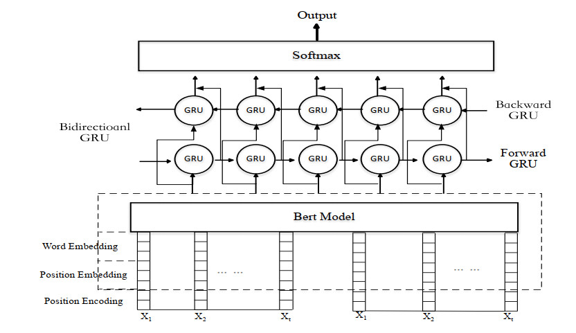
Citation: Yi Liu, Jiahuan Lu, Jie Yang, Feng Mao. Sentiment analysis for e-commerce product reviews by deep learning model of Bert-BiGRU-Softmax[J]. Mathematical Biosciences and Engineering, 2020, 17(6): 7819-7837. doi: 10.3934/mbe.2020398
[1] | Hany Bauomy, Ashraf Taha . Nonlinear saturation controller simulation for reducing the high vibrations of a dynamical system. Mathematical Biosciences and Engineering, 2022, 19(4): 3487-3508. doi: 10.3934/mbe.2022161 |
[2] | Chunguang Dong, Zhuojie Zhang, Xiaoxia Zhen, Mu Chen . Free vibration of summation resonance of suspended-cable-stayed beam. Mathematical Biosciences and Engineering, 2019, 16(6): 7230-7249. doi: 10.3934/mbe.2019363 |
[3] | Jinhua Zou, Yonghui Huang, Wenxian Feng, Yanhua Chen, Yue Huang . Experimental study on flexural behavior of concrete T-beams strengthened with externally prestressed tendons. Mathematical Biosciences and Engineering, 2019, 16(6): 6962-6974. doi: 10.3934/mbe.2019349 |
[4] | Xiaoyu Du, Yijun Zhou, Lingzhen Li, Cecilia Persson, Stephen J. Ferguson . The porous cantilever beam as a model for spinal implants: Experimental, analytical and finite element analysis of dynamic properties. Mathematical Biosciences and Engineering, 2023, 20(4): 6273-6293. doi: 10.3934/mbe.2023270 |
[5] | Yukun Song, Yue Song, Yongjun Wu . Adaptive boundary control of an axially moving system with large acceleration/deceleration under the input saturation. Mathematical Biosciences and Engineering, 2023, 20(10): 18230-18247. doi: 10.3934/mbe.2023810 |
[6] | Peng Zheng, Jingwei Gao . Damping force and energy recovery analysis of regenerative hydraulic electric suspension system under road excitation: modelling and numerical simulation. Mathematical Biosciences and Engineering, 2019, 16(6): 6298-6318. doi: 10.3934/mbe.2019314 |
[7] | Kimberly Fessel, Mark H. Holmes . A model for the nonlinear mechanism responsible for cochlear amplification. Mathematical Biosciences and Engineering, 2014, 11(6): 1357-1373. doi: 10.3934/mbe.2014.11.1357 |
[8] | Zhi Li, Jiyang Fu, Qisheng Liang, Huajian Mao, Yuncheng He . Modal identification of civil structures via covariance-driven stochastic subspace method. Mathematical Biosciences and Engineering, 2019, 16(5): 5709-5728. doi: 10.3934/mbe.2019285 |
[9] | Siyu Liu, Yong Li, Yingjie Bi, Qingdao Huang . Mixed vaccination strategy for the control of tuberculosis: A case study in China. Mathematical Biosciences and Engineering, 2017, 14(3): 695-708. doi: 10.3934/mbe.2017039 |
[10] | Nasim Ullah, Al-sharef Mohammad . Cascaded robust control of mechanical ventilator using fractional order sliding mode control. Mathematical Biosciences and Engineering, 2022, 19(2): 1332-1354. doi: 10.3934/mbe.2022061 |
The function class H(E) is a collection of the function f which are holomorphic in the open unit disc
E={z:z∈C and |z|<1}. |
Let Ap denote the class of all functions f which are analytic and p-valent in the open unit disk E and has the Taylor series expansion of the form
f(z)=zp+∞∑n=p+1anzn, (p∈N={1,2,...}). | (1.1) |
For briefly, we write as:
A1=A. |
Moreover, S represents the subclass of A which is univalent in open unit disk E. Further in area of Geometric Function Theory, numerous researchers offered their studies for the class of analytic function and its subclasses as well. The role of geometric properties is remarkable in the study of analytic functions, for instance convexity, starlikeness, close-to-convexity. A function f∈Ap is known as p-valently starlike (S∗p) and convex (Kp), whenever it satisfies the inequality
ℜ(zf′(z)f(z))>0,(z∈E) |
and
ℜ(1+zf′′(z)f′(z))>0,(z∈E). |
Moreover, a function f(z)∈Ap, is said to be p-valently starlike function of order α, written as f(z)∈S∗p(α), if and only if
ℜ(zf′(z)f(z))>α,(z∈E). |
Similarly, a function f(z)∈Ap, is said to be p-valently convex functions of order α, written as f(z)∈ Kp(α), if and only if
ℜ(1+zf′′(z)f′(z))>α,(z∈E), |
for some 0≤α<p. In particular, we have
S∗p(0)=S∗p |
and
Kp(0)=Kp. |
The convolution (Hadamard product) of f(z) and g(z) is defined as:
f(z)∗g(z)=∞∑n=0anbnzn=g(z)∗f(z), |
where
f(z)=∞∑n=0anzn and g(z)=∞∑n=0bnzn, (z∈E). |
Let P denote the well-known Carathéodory class of functions m, analytic in the open unit disk E of the form
m(z)=1+∞∑n=1cnzn, | (1.2) |
and satisfy
ℜ(m(z))>0. |
The quantum (or q-) calculus has a great important because of its applications in several fields of mathematics, physics and some related areas. The importance of q-derivative operator (Dq) is pretty recongnizable by its applications in the study of numerous subclasses of analytic functions. Initially in 1908, Jackson [14] defined the q -analogue of derivative and integral operator as well as provided some of their applications. Further in [11] Ismail et al. gave the idea of q -extension of class of q-starlike functions after that Srivastava [37] studied q-calculus in the context of univalent functions theory, also numerous mathematician studied q-calculus in the context of geometric functions theory. Kanas and Raducanu [17] introduced the q -analogue of Ruscheweyh differential operator and Arif et al. [3,4] discussed some of its applications for multivalent functions while Zhang et al. in [50] studied q-starlike functions related with generalized conic domain Ωk,α. By using the concept of convolution Srivastava et al. [40] introduced q-Noor integral operator and studied some of its applications, also Srivastava et al. published set of articles in which they concentrated class of q-starlike functions from different aspects (see [24,41,42,44,46,47]). Additionally, a recently published survey-cum-expository review article by Srivastava [38] is potentially useful for researchers and scholars working on these topics. For some more recent investigation about q -calculus we may refer to [1,18,19,20,21,22,23,25,31,32,33,34,38,39,45].
For better understanding of the article we recall some concept details and definitions of the q-difference calculus. Throughout the article we presume that
0<q<1 and p∈N={1,2,3...}. |
Definition 1. ([10]) The q-number [t]q for q∈(0,1) is defined as:
[t]q={1−qt1−q, (t∈C),n−1∑k=0qk , (t=n∈N). |
Definition 2. The q-factorial [n]q! for q∈(0,1) is defined as:
[n]q!={1, (n=0),n∏k=1[k]q , (n∈N). |
Definition 3. The q-generalized Pochhammer symbol [t]n,q, t∈C, is defined as:
[t]n,q={1, (n=0),[t]q[t+1]q[t+2]q...[t+n−1]q, (n∈N). |
And the q-Gamma function be defined as:
Γq(t+1)=[t]qΓq(t) and Γq(1)=1. |
Definition 4. The q-integral of any function f(z) was defined be Jackson [15] as follows:
∫f(z)dqz=(1−q)z∞∑n=0f(qnz)qn |
provided that the series on right hand side converges absolutely.
Definition 5. ([14]) For given q∈(0,1), the q-derivative operator or q-difference operator of f is defined by:
Dqf(z)=f(z)−f(qz)(1−q)z, z≠0,q≠1,=1+∞∑n=2[n]qanzn−1. | (1.3) |
Now we extend the idea of q-difference operator to a function f given by (1.1) from the class Ap as:
Definition 6. For f∈Ap, let the q-derivative operator (or q -difference operator) be defined as:
Dqf(z)=f(z)−f(qz)(1−q)z, z≠0,q≠1,=[p]qzp−1+∞∑n=p+1[n]qanzn−1. | (1.4) |
We can observe that for p=1, and q→1− in (1.4) we have
limq→1−Dqf(z)=f′(z). |
Definition 7. An analytic function f(z)∈S∗p(α,q) of p-valent q-starlike functions of order α in E, if f(z)∈Ap, satisfies the condition
ℜ(zDqf(z)f(z))>α,(z∈E), |
for some 0≤α<p.
Definition 8. An analytic function f(z)∈Kp(α,q) of p-valent q -convex functions of order α in E, if f(z)∈Ap, satisfies the condition
ℜ(Dq(zDqf(z))Dqf(z))>α,(z∈E), |
for some 0≤α<p.
Remark 1. Let f(z)∈Ap, it follows that
f(z)∈Kp(α,q) if and only if zDqf(z)[p]q∈S∗p(α,q) |
and
f(z)∈S∗p(α,q) if and only if z∫0[p]qf(ζ)ζdqζ∈Kp(α,q). |
Remark 2. By putting value of parameters α and p we can get some new subclasses of analytic functions:
S∗p(q)=S∗p(0,q), S∗(α,q)=S∗1(α,q), Kp(q)=Kp(0,q) and K(α,q)=K1(α,q). |
Remark 3. By taking q→1−, then we obtain two known subclasses S∗p(α) and Kp(α) of p -valently starlike and convex functions of order α, introduced by Hayami and Owa in [12].
Let n∈N0 and j∈N. The jth Hankel determinant was introduced and studied in [29]:
Hj(n)=|an an+1… an+j−1an+1 an+2…an+j−2… … …… … …an+j−1 an+j−2…an+2j−2|, |
where a1=1. The Hankel determinant H2(1) represents a Fekete-Szeg ö functional |a3−a22|. This functional has been further generalized as |a3−μa22| for some real or complex number μ and also the functional |a2a4−a23| is equivalent to H2(2) (see [16]). Babalola [5] studied the Hankel determinant H3(1) (see also [43]). The symmetric Toeplitz determinant Tj(n) is defined as follows:
Tj(n)=|an an+1… an+j−1an+1 … …… … …… … …an+j−1 … an|, | (1.5) |
so that
T2(2)=|a2 a3a3 a2|, T2(3)=|a3 a4a4 a3|, T3(2)=|a2 a3 a4a3 a2 a3a4 a3 a2| |
and so on. The problem of finding the best possible bounds for ||an+1|−|an|| has a long history (see [8]). In particular, several authors [13,44] have studied Tj(n) for several classes.
For our simplicity, we replace n=n+p−1, into (1.5), then the symmetric Toeplitz determinant Tj(n) can be written as:
Tj(n+p−1)=|an+p−1 an+p…an+p+j−2an+p … … … … …… … …an+p+j−2 … an+p−1|, |
so that
T2(p+1)=|ap+1 ap+2ap+2 ap+1|, T2(p+2)=|ap+2 ap+3ap+3 ap+2|, T3(p+1)=|ap+1 ap+2 ap+3ap+2 ap+1 ap+2ap+3 ap+2 ap+1|. |
Hankel determinants generated by perturbed Gaussian, Laguerre and Jacobi weights play an important role in Random Matrix Theory, since they represent the partition functions for the perturbed Gaussian, Laguerre and Jacobi unitary ensembles, see for example [7,26,27,28,49].
In order to discuss our problems, we need some lemmas.
Lemma 1. (see [8]). If a function m(z)=1+∞∑n=1cnzn∈P, then
|cn|≤2,n≥1. |
The inequality is sharp for
f(z)=1+z1−z. |
Lemma 2. If a function m(z)=[p]q+∞∑n=1cnzn satisfies the following inequality
ℜ(m(z))≥α |
for some α, (0≤α<p), then
|cn|≤2([p]q−α),n≥1. |
The result is sharp for
m(z)=[p]q+([p]q−2α)z1−z=[p]q+∞∑n=12([p]q−α)zn. |
Proof. Let
l(z)=m(z)−α[p]q−α=1+∞∑n=1cn[p]q−αzn. |
Noting that l(z)∈P and using Lemma 1, we see that
|cn[p]q−α|≤2, n≥1, |
which implies
|cn|≤2([p]q−α), n≥1. |
Remark 4. When q→1−, then Lemma 2, reduces to the lemma which was introduced by Hayami et al. [12].
Lemma 3. ([36]) If m is analytic in E and of the form (1.2), then
2c2=c21+x(4−c21) |
and
4c3=c31+2(4−c21)c1x−(4−c21)c1x2+2(4−c21)(1−|x2|)z, |
for some x, z∈C, with |z|≤1, and |x|≤1.
By virtue of Lemma 3, we have
Lemma 4. If m(z)=[p]q+∞∑n=1cnzn satisfy ℜ(m(z)>α, for some α (0≤α<p), then
2([p]q−α)c2=c21+{4([p]q−α)2−c21}x |
and
4([p]q−α)2c3=c31+2{4([p]q−α)2−c21}c1x−{4([p]q−α)2−c21}c1x2+2([p]q−α){4([p]q−α)2−c21}(1−|x2|)z, |
for some x, z∈C, with |z|≤1, and |x|≤1.
Proof. Since l(z)=m(z)−α[p]q−α=1+∞∑n=1cn[p]q−αzn∈P, replacing c2 and c3 by c2[p]q−αand c3[p]q−α in Lemma 3, respectively, we immediately have the relations of Lemma 4.
Remark 5. When q→1−, then Lemma 4, reduces to the lemma which was introduced by Hayami et al. [12].
Lemma 5. ([9]) Let the function m(z) given by (1.2) having positive real part in E. Also let μ∈C, then
|cn−μckcn−k|≤2max(1,|2μ−1|),1≤k≤n−k. |
Theorem 1. Let the function f given by (1.1) belong to the class S∗p(α,q), then
|ap+1|≤2([p]q−α)[p+1]q−[p]q,|ap+2|≤2([p]q−α)[p+2]q−[p]q{1+2([p]q−α)[p+1]q−[p]q},|ap+3|≤2([p]q−α)[p+3]q−[p]q[1+2([p]q−α)Λ2{ρ3+2([p]q−α)}], |
where Λ2 is given by (3.6).
Proof. Let f∈S∗(α,q), then their exist a function P(z)=[p]q+∞∑n=1cnzn such that ℜ(m(z))>α and
z(Dqf)(z)f(z)=m(z), |
which implies that
z(Dqf)(z)=m(z)f(z). |
Therefore, we have
([n]q−[p]q)an=n−1∑l=palcn−l, | (3.1) |
where n≥p+1,ap=1, c0=[p]q. From (3.1), we have
ap+1=c1[p+1]q−[p]q, | (3.2) |
ap+2=1[p+2]q−[p]q{c2+c21([p+1]q−[p]q)}, | (3.3) |
ap+3=1[p+3]q−[p]q{c3+Λ1c1c2+Λ2c31}, | (3.4) |
where
Λ1=Λ2ρ3, | (3.5) |
Λ2=1([p+1]q−[p]q)([p+2]q−[p]q), | (3.6) |
ρ3=[p+1]q+[p+2]q−2[p]q. | (3.7) |
By using Lemma 2, we obtain the required result.
Theorem 2. Let an analytic function f given by (1.1) be in the class S∗p(α,q), then
T3((p+1)≤Λ3[Ω4+4([p]q−α)2Ω5+Ω7+Ω8|1−2([p]q−α)Ω6Ω8|], |
where
Λ3=4([p]q−α)2[Ω1+Ω2(1+Ω3)],Ω1=2([p]q−α)[p+1]q−[p]q, | (3.8) |
Ω2=2([p]q−α)[p+3]q−[p]q, | (3.9) |
Ω3=2([p]q−α)Λ2{ρ3+2([p]q−α)}, | (3.10) |
Ω4=1([p+1]q−[p]q)2,Ω5=2Λ2Λ2−Λ2ρ4, | (3.11) |
Ω6=4Λ2([p+2]q−[p]q)−Λ2ρ3ρ4,Ω7=2([p+2]q−[p]q)2, | (3.12) |
Ω8=ρ4=1([p+1]q−[p]q)([p+3]q−[p]q). | (3.13) |
Proof. A detailed calculation of T3(p+1) is in order.
T3(p+1)=(ap+1−ap+3)(a2p+1−2a2p+2+ap+1ap+3), |
where ap+1, ap+2, and ap+3 is given by (3.2), (3.3) and (3.4).
Now if f∈S∗(α,q), then we have
|ap+1−ap+3|≤|ap+1|+|ap+3|, ≤ Ω1+Ω2(1+Ω3), | (3.14) |
where Ω1, Ω2, Ω3, is given by (3.9), (3.10) and (3.11).
We need to maximize |a2p+1−2a2p+2+ap+1ap+3| for f∈S∗(α,q), so by writing ap+1, ap+2, ap+3 in terms of c1,c2,c3, with the help of (3.2), (3.3) and (3.4), we get
|a2p+1−2a2p+2+ap+1ap+3|≤|Ω4c21−Ω5c41−Ω6c21c2−Ω7c22+Ω8c1c3|,≤Ω4c21+Ω5c41+Ω7c22+Ω8c1|c3−Ω6c1c2Ω8|. | (3.15) |
Finally applying Lemmas 2 and 5 along with (3.14) and (3.15), we obtained the required result.
For q→1−, p=1 and α=0, we have following known corollary.
Corollary 1. ([2]). Let an analytic function f be in the class S∗, then
T3(2)≤84. |
Theorem 3. If an analytic function f given by (1.1) belongs to the class S∗p(α,q), then
|ap+1ap+3−a2p+2|≤4([p]q−α)2([p+2]q−[p]q)2. |
Proof. Making use of (3.2), (3.3) and (3.4), we have
ap+1ap+3−a2p+2=ρ4c1c3+(Λ2ρ3−B)c21c2−Dc22+(Λ2ρ4−Λ2Λ2)c41, |
where
D=1([p+2]q−[p]q)2, B=2Λ2[p+2]q−[p]q. |
By using Lemma 3 and we take Υ=4([p]q−α)2−c21 and Z=(1−|x|2)z. Without loss of generality we assume that c=c1, (0≤c≤2([p]q−α)), so that
ap+1ap+3−a2p+2=λ1c4+λ2Υc2x−λ3Υc2x2−λ4Υ2x2+λ5ΥcZ, | (3.16) |
where
λ1=ρ44([p]q−α)2+Λ2ρ3−B2([p]q−α)−D4([p]q−α)2−D(Λ2ρ4−Λ2Λ2)4([p]q−α)2,λ2=ρ42([p]q−α)2+Λ2ρ3−B2([p]q−α)−D2([p]q−α)2,λ3=ρ44([p]q−α)2, λ4=D4([p]q−α)2, λ5=ρ42([p]q−α). |
Taking the modulus on (3.16) and using triangle inequality, we find that
|ap+1ap+3−a2p+2|≤|λ1|c4+|λ2|Υc2|x|+|λ3|Υc2|x|2+|λ4|Υ2|x|2+|λ5|(1−|x|2)cΥ=G(c,|x|). |
Now, trivially we have
G′(c,|x|)>0 |
on [0,1], which shows that G(c,|x|) is an increasing function in an interval [0,1], therefore maximum value occurs at x=1 and Max G(c,|1|)=G(c).
G(c,|1|)=|λ1|c4+|λ2|Υc2+|λ3|Υc2+|λ4|Υ2 |
and
G(c)=|λ1|c4+|λ2|Υc2+|λ3|Υc2+|λ4|Υ2. |
Hence, by putting Υ=4−c21 and after some simplification, we have
G(c)=(|λ1|−|λ2|−|λ3|+|λ4|)c4+4(|λ2|+|λ3|−2|λ4|)c2+16|λ4|. |
We consider G′(c)=0, for optimum value of G(c), which implies that c=0. So G(c) has a maximum value at c=0. Hence the maximum value of G(c) is given by
16|λ4|. | (3.17) |
Which occurs at c=0 or
c2=4(|λ2|+|λ3|−2|λ4|)|λ1|−|λ2|−|λ3|+|λ4|. |
Hence, by putting λ4=D4([p]q−α)2 and D=1([p+2]q−[p]q)2 in (3.17) and after some simplification, we obtained the desired result.
For q→1−, p=1 and α=0, we have following known corollary.
Corollary 2. ([16]). If an analytic function f belongs to the class S∗, then
|a2a4−a23|≤1. |
Theorem 4. Let f be the function given by (1.1) belongs to the class S∗p(α,q), 0≤α<p, then
|ap+2−μa2p+1|≤{2([p]q−α)([p+2]q−[p]q){ρ1−ρ2μ},if μ≤ρ5,2([p]q−α)([p+2]q−[p]q), if ρ5≤μ≤ρ6,2([p]q−α)([p+1]q−[p]q)2([p+2]q−[p]q){ρ2μ−ρ1},if μ≥ρ6, |
where
ρ1={2([p]q−α)([p+1]q−[p]q)+([p+1]q−[p]q)2},ρ2=2([p]q−α)([p+2]q−[p]q),ρ5=([p+1]q−[p]q){2([p]q−α)+([p+1]q−[p]q)}−12([p]q−α)([p+2]q−[p]q),ρ6=([p+1]q−[p]q)([p]q−α+([p+1]q−[p]q))([p]q−α)([p+2]q−[p]q). |
Proof. From (3.2) and (3.3) and we can suppose that c1=c (0≤c≤2([p]q−α)), without loss of generality we derive
|ap+2−μa2p+1|=1ρ7|{ρ1−ρ2μ}c2+([p+1]q−[p]q)2{4([p]q−α)2−c2}ρ|=A(ρ), |
where
ρ7=2([p]q−α)([p+1]q−[p]q)2([p+2]q−[p]q). |
Applying the triangle inequality, we deduce
A(ρ)≤1ρ7|{ρ1−ρ2μ}|c2+([p+1]q−[p]q)2{4([p]q−α)2−c2}={1ρ7[{2([p]q−α){ρ11−ρ12μ}}c2+ρ9], if μ≤ρ8,1ρ7[2{([p]q−α)([p+2]q−[p]q)μ−ρ10}c2+ρ9], if μ≥ρ8, |
where
ρ8=2([p]q−α)([p+1]q−[p]q)+([p+1]q−[p]q)22([p]q−α)([p+2]q−[p]q),ρ9=4([p]q−α)2([p+1]q−[p]q)2,ρ10=([p+1]q−[p]q){([p]q−α)+([p+1]q−[p]q)},ρ11=([p+1]q−[p]q),ρ12=([p+2]q−[p]q),ρ13=2([p]q−α)([p+1]q−[p]q)2([p+2]q−[p]q). |
|ap+2−μa2p+1|≤{2([p]q−α)([p+2]q−[p]q){ρ1−ρ2μ},if μ≤ρ5, c=2([p]q−α),2([p]q−α)([p+2]q−[p]q),if ρ5≤μ≤ρ8,c=0,2([p]q−α)([p+2]q−[p]q),if ρ8≤μ≤ρ6,c=0,ρ13{ρ2μ−{2([p]q−α)ρ11+ρ211}}, if μ≥ρ6,c=2([p]q−α). |
If q→1− in Theorem 4, we thus obtain the following known result.
Corollary 3. ([12]). Let f be the function given by (1.1) belongs to the class S∗p(α), 0≤α<p, then
|ap+2−μa2p+1|≤{(p−α){{2(p−α)+1}−4(p−α)μ},if μ≤12,(p−α), if 12≤μ≤p−α+12(p−α),(p−α){4(p−α)μ−{2(p−α)+1}},if μ≥p−α+12(p−α). |
In this section, firstly we recall that the q-Bernardi integral operator for multivalent functions L(f)=Bqp,β given in [35] as:
Let f∈Ap, then L:Ap→Ap is called the q-analogue of Benardi integral operator for multivalent functions defined by L(f)=Bqq,β with β>−p, where, Bqq,β is given by
Bqp,βf(z)=[p+β]qzβ∫z0tβ−1f(t)dqt, | (3.18) |
=zp+∞∑n=1[β+p]q[n+β+p]qan+pzn+p, z∈E,=zp+∞∑n=1Bn+pan+pzn+p. | (3.19) |
The series given in (3.19) converges absolutely in E.
Remark 6. For q→1−, then the operator Bqp,β reduces to the integral operator studied in [48].
Remark 7. For p=1, we obtain the q-Bernardi integral operator introduced in [30].
Remark 8. If q→1− and p=1, we obtain the familiar Bernardi integral operator studied in [6].
Theorem 5. If f is of the form (1.1), belongs to the class S∗p(α,q), and
Bqp,βf(z)=zp+∞∑n=1Bn+pan+pzn+p, |
where Bqp,β is the integral operator given by (3.18), then
|ap+1|≤2([p]q−α)([p+1]q−[p]q)Bp+1,|ap+2|≤2([p]q−α)([p+2]q−[p]q)Bp+2{1+2([p]q−α)([p+1]q−[p]q)Bp+1},|ap+3|≤2([p]q−α)([p+3]q−[p]q)Bp+3[1+2([p]q−α)ρ14ρ15], |
where
ρ14={(([p+1]q−[p]q)Bp+1+([p+2]q−[p]q)Bp+2)+2([p]q−α)},ρ15=([p+1]q−[p]q)([p+2]q−[p]q)Bp+1Bp+2. |
Proof. The proof follows easily by using (3.19) and Theorem 1.
Theorem 6. Let an analytic function f given by (1.1) be in the class S∗p(α,q), in addition Bqp,β is the integral operator defined by (3.18) and is of the form (3.19), then
T3((p+1)≤Υ3[Ω4B2p+1+4([p]q−α)2Ω10+Ω7B2p+2+Ω8Bp+1Bp+3|1−2([p]q−α)Bp+1Bp+3Ω11Ω8|], |
where
Υ3=4([p]q−α)2[Ω1Bp+1+Ω2Bp+3(1+Ω9)],Ω9=Λp(ρ14Bp+1Bp+2),Ω10=Λ4−Λ5,Ω11=Λ6−Λ7, |
Λ4=2Λ2Λ2B2p+1B2p+2,Λ5=Λ2ρ4B2p+1Bp+2Bp+3,Λ6=4Λ2([p+2]q−[p]q)Bp+1B2p+2,Λ7=Λ8Λ2ρ4B2p+1Bp+2Bp+3,Λ8=([p+1]q−[p]q)Bp+1+([p+2]q−[p]q)Bp+2. |
Proof. The proof follows easily by using (3.19) and Theorem 2.
Theorem 3. If an analytic function f given by (1.1) belongs to the class S∗p(α,q), in addition Bqp,β is the integral operator is defined by (3.18) and is of the form (3.19), then
|ap+1ap+3−a2p+2|≤4([p]q−α)2([p+2]q−[p]q)2B2p+2. |
Theorem 8. Let f be the function given by (1.1) belongs to the class S∗p(α,q), in addition Bqp,β is the integral operator defined by (3.18) and is of the form (3.19), then
|ap+2−μa2p+1|≤{2([p]q−α)([p+2]q−[p]q)Bp+2{ρ16−ρ2Bp+2μ},if μ≤ρ17,2([p]q−α)([p+2]q−[p]q)Bp+2,if ρ17≤μ≤ρ18,2Λ2([p]q−α)([p+1]q−[p]q)B2p+1Bp+2{ρ2Bp+2μ−ρ16},if μ≥ρ18, |
where
ρ16={2([p]q−α)([p+1]q−[p]q)Bp+1+([p+1]q−[p]q)2B2p+1},ρ17=([p+1]q−[p]q)Bp+1{2([p]q−α)+([p+1]q−[p]q)Bp+1}−12([p]q−α)([p+2]q−[p]q)Bp+2,ρ18=([p+1]q−[p]q)Bp+1([p]q−α+([p+1]q−[p]q)Bp+1)([p]q−α)([p+2]q−[p]q)Bp+2, |
and Λ2 is given by (3.6).
Motivated by a number of recent works, we have made use of the quantum (or q-) calculus to define and investigate new subclass of multivalent q -starlike functions in open unit disk E. We have studied about Hankel determinant, Toeplitz matrices, Fekete–Szegö inequalities. Furthermore we discussed applications of our main results by using q-Bernardi integral operator for multivalent functions. All the results that have discussed in this paper can easily investigate for the subclass of meromorphic q-convex functions (Kp(α,q)) of order α in E, respectively.
Basic (or q-) series and basic (or q-) polynomials, especially the basic (or q-) hypergeometric functions and basic (or q-) hypergeometric polynomials, are applicable particularly in several diverse areas (see [38], p328). Moreover, in this recently-published survey-cum expository review article by Srivastava [38], the so called (p,q)-calculus was exposed to be a rather trivial and inconsequential variation of the classical q-calculus (see for details [38], p340).
By this observation of Srivastava in [38], we can make clear link between the q-analysis and (p,q)-analysis and the results for q -analogues which we have included in this paper for 0<q<1, can be easily transformed into the related results for the (p,q)-analogues with (0<q<p≤1).
This work is supported by the program for Young Talents of Science and Technology in Universities of Inner Mongolia Autonomous Region under the Grant NJYT-18-A14, the Natural Science Foundation of Inner Mongoliaof the people's Republic of China under Grant 2018MS01026, the Natural Science Foundation of the people's Republic of China under Grant 11561001.
The authors declare that they have no competing interests.
[1] |
P. Sasikala, L. M. I. Sheela, Sentiment analysis of online product reviews using DLMNN and future prediction of online product using IANFIS, J. Big Data, 7 (2020), 33-53. doi: 10.1186/s40537-020-00308-7
![]() |
[2] |
P. A. Pavlou, A. Dimoka, The nature and role of feedback text comments in online marketplaces: Implications for trust building, price premiums, and seller differentiation, Inf. Syst. Res., 17 (2006), 392-414. doi: 10.1287/isre.1060.0106
![]() |
[3] | A. Abbasi, H. Chen, A. Salem, Sentiment analysis in multiple languages: feature selection for opinion classification in web forums, ACM Trans. Inf. Syst., 26 (2008), 12-21. |
[4] | Z. Zhang, Y. E. Qiang, Literature review on sentiment analysis of online product reviews, J. Manage. Sci. China, 13 (2010), 84-96. |
[5] | C. Chang, C. J. Lin, LIBSVM: A library for support vector machines, ACM Trans. Intel. Syst. Technol., 2 (2011), 1-27. |
[6] |
F. Hu, L. Li, Z. L. Zhang, et al, Emphasizing essential words for sentiment classification based on recurrent neural networks, J. Comput. Sci. Technol., 32 (2017), 785-795. doi: 10.1007/s11390-017-1759-2
![]() |
[7] | Y. Mejova, P. Srinivasan, Exploring feature definition and selection for sentiment classifiers. In Proc. 5th Int. Conf. weblogs social media, Barcelona, Catalonia, Spain, (2011), 17-21. |
[8] | W. Casey, G. Navendu, A. Shlomo, Using appraisal groups for sentiment analysis. In Proc. ACM SIGIR Conf. Inform. Knowl. Manag., (2005), 625-31. |
[9] |
L.-C. Yu, H.-L. Wu, P.-C. Chang, H.-S. Chu, Using a contextual entropy model to expand emotion words and their intensity for the sentiment classification of stock market news, Knowl. Based Syst., 41 (2013), 89-97. doi: 10.1016/j.knosys.2013.01.001
![]() |
[10] | I. Jolliffe, N. A. Jolliffe, Principal Component Analysis. Springer Series in Statistics, 2nd edition, Springer-Verlag, New York, 2002. |
[11] |
D. Adnan, F. Song, Feature selection for sentiment analysis based on content and syntax models, Decis. Support Syst., 53 (2012), 704-11. doi: 10.1016/j.dss.2012.05.023
![]() |
[12] | L. G. Thomas, S. Mark, M. B. David, B. T. Joshua, Integrating topics and syntax, Adv. Neural Inf. Process. Syst., (2005), 537-544. |
[13] |
A. Yadav, D. K. Vishwakarma, Sentiment analysis using deep learning architectures: a review, Artif. Intell. Rev., 53 (2020), 4335-4385. doi: 10.1007/s10462-019-09794-5
![]() |
[14] | S. Kim, E. Hovy, Determining the sentiment of opinions. In Proc. Conf. Comput. Linguis., Geneva, Switzerland, (2004), 1367-1373. |
[15] |
P. D. Turney, M. L. Littman, Measuring praise and criticism: Inference of semantic orientation from association, ACM Trans. Inf. Syst., 21 (2003), 315-346. doi: 10.1145/944012.944013
![]() |
[16] | Y. L. Zhu, J. Min, Y. Q. Zhou, Semantic orientation computing based on HowNet, J. Chin. Inf. Process., 20 (2006), 14-20. |
[17] | G. Somprasertsri, P. Lalitrojwong, Mining feature-opinion in online customer reviews for opinion summarization, J. Univ. Comput. Sci., 16 (2010), 938-955. |
[18] | B. Liu, Sentiment analysis and opinion mining, Synth. Lect. Hum. Lang. Technol., 5 (2012), 1-167. |
[19] | B. Pang, L. Lee, S. Vaithyanathan, Thumbs up? sentiment classification using machine learning techniques. In Proc. Conf. Empir. Methods Nat. Lang. Process., Philadelphia, USA, (2002), 79-86. |
[20] | A. Go, R. Bhayani, L. Huang, Twitter sentiment classification using distant supervision, CS224N Project Report, Stanford, 1 (2009), 1-12. |
[21] | M. Guerini, L. Gatti, M. Turchi, Sentiment analysis: How to derive prior polarities from SentiWord Net, arXiv preprint arXiv: 1309.5843. |
[22] |
A. Tripathy, A. Agrawal, S. K. Rath, Classification of sentiment reviews using n-gram machine learning approach, Expert Syst. Appl., 57 (2016), 117-126. doi: 10.1016/j.eswa.2016.03.028
![]() |
[23] | Y. KIM, Convolutional neural networks for sentence classification, arXiv preprint arXiv: 1408.5882. |
[24] | K. Cho, B. van Merrienboer, D. Bahdanau, On the properties of neural machine translation: encoder-decoder approaches. In Proce. Eighth Workshop Syntax, Semant. Struct. Stat. Trans., Doha, Qatar, (2014), 103-111. |
[25] | Z. Qu, Y. Wang, X. Wang, A Hierarchical attention network sentiment classification algorithm based on transfer learning, J. Comput. Appl., 38 (2018), 3053-3056. |
[26] | J. Pennington, R. Socher, C. D. Manning, GloVe: Global vectors for word representation, Proc. Int. Conf. Empir. Methods Nat. Lang. Process., (2014), 147-168. |
[27] |
F. Abid, M. Alam, M. Yasir, C. Li, Sentiment analysis through recurrent variants latterly on convolutional neural network of twitter, Future Gener. Comput. Syst., 95 (2019), 292-308. doi: 10.1016/j.future.2018.12.018
![]() |
[28] | J. Trofimovich, Comparison of neural network architectures for sentiment analysis of Russian tweets, In Proc. Int. Conf. Dialogue 2016, RGGU, (2016). |
[29] | Q. Qian, M. Huang, J. Lei, X. Zhu, Linguistically regularized LSTMs for sentiment classification. In Proc. 55th Ann. Meet. Assoc. Comput. Ling., 1 (2016), 1679-1689. |
[30] | L. Nio, K. Murakami, Japanese sentiment classification using bidirectional long short-term memory recurrent neural network. In Proc. 24th Ann. Meeti. Assoc. Nat. Lang. Process., Okayama, Japan, (2018), 1119-1122. |
[31] |
M.-L. Zhang, Z.-H. Zhou, A review on multi-label learning algorithms, IEEE Trans. Knowl. Data Eng., 26 (2014), 1819-1837. doi: 10.1109/TKDE.2013.39
![]() |
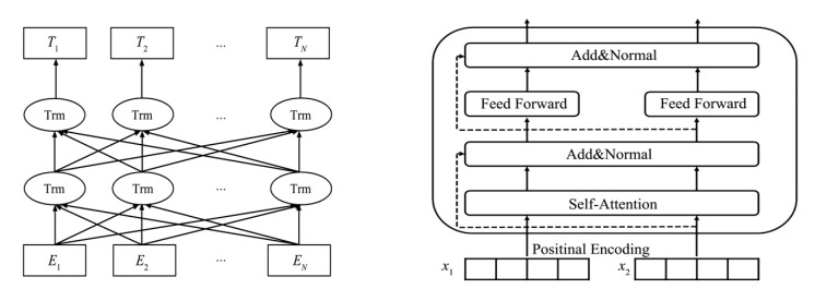
[32] | J. Devlin, M. W. Chang, K. Lee, K. Toutanova, BERT: Pre-Training of deep bidirectional transformers for language understanding, In Proc. 2019 Conf. North Am. Chapter Assoc. Comput. Linguist. Human Lang. Tech., (2019), 4171-4186. |
[33] |
S. Seo, C. Kim, H. Kim, et al, Comparative study of deep learning based sentiment classification, IEEE Access, 8 (2020), 6861-6875. doi: 10.1109/ACCESS.2019.2963426
![]() |
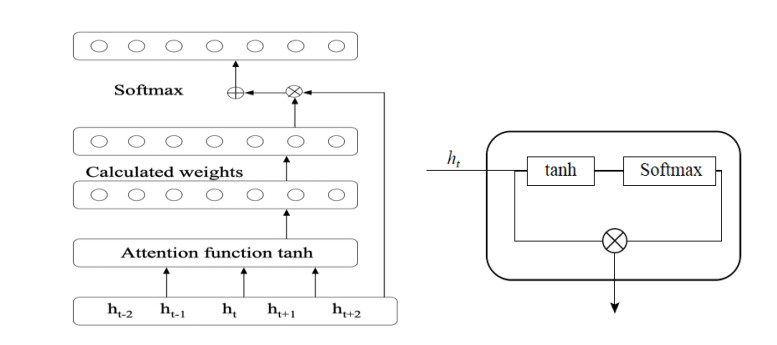
[34] | B. Dzmitry, C. Kyunghyun, B. Yoshua, Neural machine translation by jointly learning to align and translate, In Proc. Int. Conf. Learn. Representations 2015, San Diego, CA, USA, (2015), 1-15. |
[35] | D. Li, F. Wei, C. Tan, Adaptive recursive neural network for target-dependent twitter sentiment classification, Baltimore: Assoc. Comput. Ling.-ACL, (2014), 49-54. |
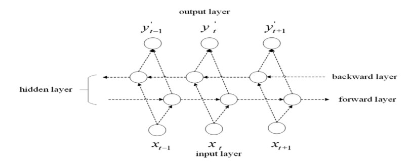
[36] | S. M. Grü.er-Sinopoli, C. N. Thalemann, Bidirectional recurrent neural networks, IEEE Trans. Signal Process., 11 (1997), 2673-2681 |
[37] |
S. Zhang, X. Xu, Y. Pang, J. Han, Multi-layer Attention Based CNN for Target-Dependent Sentiment Classification, Neural Process. Lett., 51 (2020), 2089-2103 doi: 10.1007/s11063-019-10017-9
![]() |
[38] | K. Saranya, S. Jayanthy, Onto-based sentiment classification using machine learning techniques. In Proc. 2017 Int. Conf. Innovations Inf., Embed. Commun. Syst., (2017), 1-5. |
[39] |
S. Tan, J. Zhang, An empirical study of sentiment analysis for Chinese documents, Expert Syst. Appl., 34 (2008), 2622-2629. doi: 10.1016/j.eswa.2007.05.028
![]() |
[40] | W. Li, F. Qi, Sentiment analysis based on multi-channel bidirectional long short term memory network, J. Chin. Inf. Process., 33 (2019), 119-128. |
[41] | Y. Yang, H. Yuan, Y. Wang, Sentiment analysis method for comment text, J. Nanjing Univ. Sci. Tech., 43 (2019), 280-285. |
1. | Khalid Alluhydan, Yasser A. Amer, Ashraf Taha EL-Sayed, Marwa A. EL-Sayed, Controlling the Generator in a Series of Hybrid Electric Vehicles Using a Positive Position Feedback Controller, 2024, 14, 2076-3417, 7215, 10.3390/app14167215 | |
2. | Celia Hameury, Giovanni Ferrari, Giulio Franchini, Marco Amabili, An experimental approach to multi-input multi-output nonlinear active vibration control of a clamped sandwich beam, 2024, 216, 08883270, 111496, 10.1016/j.ymssp.2024.111496 | |
3. | Khalid Alluhydan, Yasser A. Amer, Ashraf Taha EL-Sayed, Marwa Abdelaziz EL-Sayed, The Impact of the Nonlinear Integral Positive Position Feedback (NIPPF) Controller on the Forced and Self-Excited Nonlinear Beam Flutter Phenomenon, 2024, 16, 2073-8994, 1143, 10.3390/sym16091143 | |
4. | Ruihai Geng, Yunfeng Bai, Chunyang Shi, Jiale Peng, Yushu Bian, Primary resonance control of flexible manipulator based on modal coupling and time-delay feedback, 2025, 13, 2195-268X, 10.1007/s40435-024-01579-1 |