Loading [MathJax]/jax/output/SVG/jax.js
Review Special Issues

What is the role of histone H1 heterogeneity? A functional model emerges from a 50 year mystery

  • For the past 50 years, understanding the function of histone H1 heterogeneity has been mired in confusion and contradiction. Part of the reason for this is the lack of a working model that tries to explain the large body of data that has been collected about the H1 subtypes so far. In this review, a global model is described largely based on published data from the author and other researchers over the past 20 years. The intrinsic disorder built into H1 protein structure is discussed to help the reader understand that these histones are multi-conformational and adaptable to interactions with different targets. We discuss the role of each structural section of H1 (as we currently understand it), but we focus on the H1's C-terminal domain and its effect on each subtype's affinity, mobility and compaction of chromatin. We review the multiple ways these characteristics have been measured from circular dichroism to FRAP analysis, which has added to the sometimes contradictory assumptions made about each subtype. Based on a tabulation of these measurements, we then organize the H1 variants according to their ability to condense chromatin and produce nucleosome repeat lengths amenable to that compaction. This subtype variation generates a continuum of different chromatin states allowing for fine regulatory control and some overlap in the event one or two subtypes are lost to mutation. We also review the myriad of disparate observations made about each subtype, both somatic and germline specific ones, that lend support to the proposed model. Finally, to demonstrate its adaptability as new data further refines our understanding of H1 subtypes, we show how the model can be applied to experimental observations of telomeric heterochromatin in aging cells.

    Citation: Missag Hagop Parseghian. What is the role of histone H1 heterogeneity? A functional model emerges from a 50 year mystery[J]. AIMS Biophysics, 2015, 2(4): 724-772. doi: 10.3934/biophy.2015.4.724

    Related Papers:

    [1] Sudarshan Tiwari, Axel Klar, Giovanni Russo . Interaction of rigid body motion and rarefied gas dynamics based on the BGK model. Mathematics in Engineering, 2020, 2(2): 203-229. doi: 10.3934/mine.2020010
    [2] Jana Kopfová, Petra Nábělková . Thermoelastoplastic oscillator with Prandtl-Ishlinskii operator. Mathematics in Engineering, 2025, 7(3): 264-280. doi: 10.3934/mine.2025012
    [3] Raimondo Penta, Ariel Ramírez-Torres, José Merodio, Reinaldo Rodríguez-Ramos . Effective governing equations for heterogenous porous media subject to inhomogeneous body forces. Mathematics in Engineering, 2021, 3(4): 1-17. doi: 10.3934/mine.2021033
    [4] Thomas J. Radley, Paul Houston, Matthew E. Hubbard . Quadrature-free polytopic discontinuous Galerkin methods for transport problems. Mathematics in Engineering, 2024, 6(1): 192-220. doi: 10.3934/mine.2024009
    [5] Jinghong Li, Hongyu Liu, Wing-Yan Tsui, Xianchao Wang . An inverse scattering approach for geometric body generation: a machine learning perspective. Mathematics in Engineering, 2019, 1(4): 800-823. doi: 10.3934/mine.2019.4.800
    [6] Francesco Maddalena, Danilo Percivale, Franco Tomarelli . Signorini problem as a variational limit of obstacle problems in nonlinear elasticity. Mathematics in Engineering, 2024, 6(2): 261-304. doi: 10.3934/mine.2024012
    [7] Michael Herrmann, Karsten Matthies . Solitary waves in atomic chains and peridynamical media. Mathematics in Engineering, 2019, 1(2): 281-308. doi: 10.3934/mine.2019.2.281
    [8] Tiziano Penati, Veronica Danesi, Simone Paleari . Low dimensional completely resonant tori in Hamiltonian Lattices and a Theorem of Poincaré. Mathematics in Engineering, 2021, 3(4): 1-20. doi: 10.3934/mine.2021029
    [9] G. Gaeta, G. Pucacco . Near-resonances and detuning in classical and quantum mechanics. Mathematics in Engineering, 2023, 5(1): 1-44. doi: 10.3934/mine.2023005
    [10] Diogo Gomes, Julian Gutierrez, Ricardo Ribeiro . A mean field game price model with noise. Mathematics in Engineering, 2021, 3(4): 1-14. doi: 10.3934/mine.2021028
  • For the past 50 years, understanding the function of histone H1 heterogeneity has been mired in confusion and contradiction. Part of the reason for this is the lack of a working model that tries to explain the large body of data that has been collected about the H1 subtypes so far. In this review, a global model is described largely based on published data from the author and other researchers over the past 20 years. The intrinsic disorder built into H1 protein structure is discussed to help the reader understand that these histones are multi-conformational and adaptable to interactions with different targets. We discuss the role of each structural section of H1 (as we currently understand it), but we focus on the H1's C-terminal domain and its effect on each subtype's affinity, mobility and compaction of chromatin. We review the multiple ways these characteristics have been measured from circular dichroism to FRAP analysis, which has added to the sometimes contradictory assumptions made about each subtype. Based on a tabulation of these measurements, we then organize the H1 variants according to their ability to condense chromatin and produce nucleosome repeat lengths amenable to that compaction. This subtype variation generates a continuum of different chromatin states allowing for fine regulatory control and some overlap in the event one or two subtypes are lost to mutation. We also review the myriad of disparate observations made about each subtype, both somatic and germline specific ones, that lend support to the proposed model. Finally, to demonstrate its adaptability as new data further refines our understanding of H1 subtypes, we show how the model can be applied to experimental observations of telomeric heterochromatin in aging cells.


    A huge number of important problems in physics, astronomy, chemistry, etc. are modeled via sets of ordinary differential equations (ODEs) governed by the Hamiltonian formalism. Due to non-integrability, the investigation of the time evolution of these problems, and generally their properties, often rely solely on numerical techniques. As modern research requires numerical simulations to be pushed to their very limit (e.g., large integration times, macroscopic limits), a methodical assessment of the properties of different numerical methods becomes a fundamental issue. Such studies allow to highlight the most suitable scheme for both general purposes and specific tasks, according to criteria of stability, accuracy, simplicity and efficiency.

    The beginning of the era of computational physics is considered to be the computer experiment performed in the 1950s by Fermi, Pasta, Ulam and Tsingou (FPUT) [1,2,3] to observe energy equipartition due to weak-anharmonic coupling in a set of harmonic oscillators. Indeed, the breaking of integrability in Hamiltonian systems is often performed with the introduction of nonlinear terms in the equations of motion. These additional nonlinear terms describe new physical processes, and led to important questions and significant advancements in condensed matter physics. For instance, the FPUT problem has been used to answer questions related to ergodicity, dynamical thermalization and chaos occurrence (see e.g., [4,5,6] and references therein) and led to the observation of solitons [7,8], and progress in Hamiltonian chaos [9]. The interested reader can find a concise review of numerical results concerning the FPUT system in [10].

    Another important example concerns disordered media. In 1958, Anderson [11] theoretically showed the appearance of energy localization in one-dimensional lattices with uncorrelated disorder (a phenomenon which is now referred to as Anderson localization). This phenomenon was later investigated also for two-dimensional lattices [12]. An important question which has attracted wide attention in theory, numerical simulations and experiments is what happens when nonlinearity (which appears naturally in real world problems) is introduced in a disordered system [13,14,15,16,17,18,19,20,21,22,23,24,25,26,27,28,29,30].

    Two basic Hamiltonian models are at the center of these investigations: the disordered Klein-Gordon (DKG) chain and the disordered, discrete nonlinear Schrödinger equation (DDNLS). In Refs. [22,23,24,25,26,28,29,30,31,32,33,34] it was shown that Anderson localization is destroyed by the presence of nonlinearity, resulting to the subdiffusive spreading of energy due to deterministic chaos. Such results rely on the accurate, long time integration of the systems' equations of motion and variational equations. We note that the variational equations are a set of ODEs describing the time evolution of small deviations from a given trajectory, something which is needed for the computation of chaos indicators like the maximum Lyapunov exponent (mLE) [35,36,37]. The numerical integration of these sets of ODEs can be performed by any general purpose integrator. For example Runge-Kutta family schemes are still used [38,39]. Another category of integrators is the so-called symplectic integrators (SIs), which were particularly designed for Hamiltonian systems (see e.g., [40,41,42,43,44] and references therein). The main characteristic of SIs is that they conserve the symplectic structure of Hamiltonian systems, so that the numerical approximation they provide corresponds to the exact solution of a system which can be considered as a perturbation of the original one. Consequently the error in the computed value of the Hamiltonian function (usually refereed to as the system's energy) is kept almost constant over long integration times. This almost constant error can be used as an indicator of the accuracy of the used integration scheme.

    SIs have been successfully implemented for the long time integration of multidimensional Hamiltonian systems like the $ \alpha $- and $ \beta $-FPUT systems and FPUT-like models, the DKG, the DDNLS and systems of coupled rotors (see e.g., [22,23,24,25,26,28,29,30,32,33,45,46,47,48,49,50,51,52,53,54]). In these studies SIs belonging to the so-called SABA family [55] were mostly used, since the FPUT, the DKG and systems of coupled rotors can be split into two integrable parts (the system's kinetic and the potential energy), while in some more recent studies [33,56] the $ ABA864 $ [57] SI was implemented as it displayed an even better performance. As the DDNLS model is not explicitly decomposed into two integrable parts, the implementation of SABA schemes requires a special treatment involving the application of fast Fourier transforms which are computationally time consuming [29]. In [49,50] it was shown that for the DDNLS model, the split of the Hamiltonian function into three integrable parts is possible, and this approach proved to be the best choice for the model's integration with respect to both speed and accuracy. It is worth noting here that the numerical integration of the variational equations by SIs is done by the so-called Tangent Map Method [58,59,60].

    The intention of this work is to present several efficient (symplectic and non-symplectic) integration techniques for the time evolution of both the equations of motion and the variational equations of multidimensional Hamiltonian systems. In particular, in our study we use these techniques to investigate the chaotic dynamics of the one-dimensional (1D) FPUT system, as well as one- and two-dimensional (2D) DDNLS models. We carry out this task by considering particular initial conditions for both the systems and for the deviation vectors, which we evolve in time requiring a predefined level of energy accuracy. Then, we record the needed CPU time to perform these numerical simulations and highlight those methods that ensure the smallest CPU times for obtaining accurate results. A similar analysis for the 1D and 2D DKG systems was performed in [56].

    The paper is organized as follows. In Section 2 we introduce the models considered in our study. In Section 3 we introduce in detail the symplectic and non-symplectic schemes implemented in our investigations. In Section 4 we present our numerical results and report on the efficiency of each studied scheme. In Section 5 we review our findings and discuss the outcomes of our study. Finally, in Appendix B we provide the explicit forms of the used tangent map operators. Moreover, we present there the explicit expressions of the tangent map operators for some additional important many-body systems, the so-called $ \beta $-FPUT chain, the KG system and the classical XY model (a Josephson junction chain-JJC) in order to facilitate the potential application of SIs for these systems from the interested reader, although we do not present numerical results for these models.

    In this work we focus our analysis on the 1D FPUT system and the 1D and 2D DDNLS models. In what follows we briefly present the Hamiltonian functions of these systems.

    The 1D FPUT model [1,2,3] was first introduced in 1955 to study the road toward equilibrium of a chain of harmonic oscillators in the presence of weak anharmonic interactions. Since then, this system has been widely used as a toy model for investigating energy equipartition and chaos in nonlinear lattices. In the literature there exist two types of the FPUT model the so-called $ \alpha $- and $ \beta $-FPUT systems. In our study we consider the $ \alpha $-FPUT model whose Hamiltonian function reads

    $ H1F=Ni=0[p2i2+12(qi+1qi)2+α3(qi+1qi)3]. $ (2.1)

    In Eq.(2.1), $ q_i $ and $ p_i $ are respectively the generalized coordinates and momenta of the $ i $ lattice site and $ \alpha $ is a real positive parameter. In our study we consider fixed boundary conditions $ q_0 = p_0 = p_{N+1} = q_{N+1} = 0 $. We also note that this model conserves the value of the total energy $ H_{\text{1F}} $.

    In contrast to the $ \alpha $-FPUT system, the $ \beta $-FPUT model is characterized by a quartic nonlinear term [see Eq. (A.26) in Appendix B.4]. The fact that the value of the Hamiltonian function of the $ \beta $-FPUT model is bounded from below leads to differences between the two models. For example, phenomena of chopping time which occur in the $ \alpha $- model do not appear in the $ \beta $-FPUT system [61]. Further discussion of the differences between the $ \alpha $- and the $ \beta $- models can be found in [62,63,64].

    The DDNLS model describes anharmonic interactions between oscillators in disordered media and has been used to study the propagation of light in optical media or Bose-Einstein condensates through the famous Gross-Pitaevskii equation [52], as well as investigate, at a first approximation, several physical processes (e.g., electron tight binding systems [39]). The Hamiltonian function of the 1D DDNLS model reads

    $ H1D=Ni=1[ϵi2(q2i+p2i)+β8(q2i+p2i)2pi+1piqi+1qi], $ (2.2)

    where $ q_i $ and $ p_i $ are respectively the generalized coordinates and momenta of the $ i $ lattice site and the onsite energy terms $ \epsilon _i $ are uncorrelated numbers uniformly distributed in the interval $ \left[-\frac{W}{2}, \frac{W}{2} \right] $. The real, positive numbers $ W $ and $ \beta $ denote the disorder and the nonlinearity strength respectively. We also consider here fixed boundary conditions i.e., $ q_0 = p_0 = p_{N+1} = q_{N+1} = 0 $.

    The two-dimensional version of the DDNLS model was considered in [30,65]. Its Hamiltonian function is

    $ H2D=Ni=1Mj=1{ϵi,j2[q2i,j+p2i,j]+β8[q2i,j+p2i,j]2[qi,j+1qi,j+qi+1,jqi,j+pi,j+1pi,j+pi+1,jpi,j]}, $ (2.3)

    where $ q_{i, j} $ and $ p_{i, j} $ are respectively the generalized positions and momenta at site $ (i, j) $ and $ \epsilon _{i, j} $ are the disorder parameters uniformly chosen in the interval $ \left[-\frac{W}{2}, \frac{W}{2}\right] $. We again consider fixed boundary conditions i.e., $ q_{0, j} = p_{0, j} = q_{N+1, j} = p_{N+1, j} = 0 $ for $ 1\leq j\leq M $ and $ q_{i, 0} = p_{i, 0} = q_{i, M+1} = p_{i, M+1} = 0 $ for $ 1\leq i\leq N $.

    Additionally to the energies $ H_{1D} $ [Eq. (2.2)] and $ H_{2D} $ [Eq. (2.3)] both systems conserve their respective norms $ S_{\text{1D}} $ and $ S_{\text{2D}} $:

    $ S1D=12Ni=1(q2i+p2i) ;S2D=12Ni=1Mj=1(q2i,j+p2i,j) . $ (2.4)

    The Hamilton equations of motion

    $ dqdt=Hp ,dpdt=Hq, $ (3.1)

    of the $ N $ degree of freedom (dof) Hamiltonian $ H = H(\boldsymbol{ q}, \boldsymbol{ p}) $, with $ \boldsymbol{ q} = (q_1, q_2, \ldots, q_N) $ and $ \boldsymbol{ p} = (p_1, p_2, \ldots, p_N) $ being respectively the system's generalized positions and momenta, can be expressed in the general setting of first order ODEs as

    $ dxdt=˙x=J2NDH(x(t)), $ (3.2)

    where $ \boldsymbol{ x} = \left(\boldsymbol{ q}, \boldsymbol{ p} \right) = (x_1, x_2, \ldots, x_{N}, x_{N+1}, \ldots, x_{2N}) = (q_1, q_2, \ldots, q_N, p_1, p_2, \ldots, p_N) $ is a vector representing the position of the system in its phase space and $ (\, \dot{}\, ) $ denotes differentiation with respect to time $ t $. In Eq. (3.2)

    $ J2N=[ONININON], $ (3.3)

    is the symplectic matrix with $ \boldsymbol{I}_N $ and $ \boldsymbol{O}_N $ being the $ N\times N $ identity and the null matrices respectively, and

    $ DH=[Hq1,,HqN,Hp1,,HpN]T, $ (3.4)

    with $ (^T) $ denoting the transpose matrix.

    The variational equations (see for example [37,58]) govern the time evolution of a small perturbation $ \boldsymbol{ w}(t) $ to the trajectory $ \boldsymbol{ x}(t) $ with $ \boldsymbol{w}(t) = (\delta \boldsymbol{q}(t), \delta \boldsymbol{p}(t)) = \left(\delta q_1 (t), \delta q_2 (t), \ldots, \delta q_N (t), \delta p_1(t), \delta p_2(t), \ldots, \delta p_N (t) \right) $ (which can also be written as $ \boldsymbol{w}(t) = \delta \boldsymbol{x}(t) = \left(\delta x_1 (t), \ldots, \delta x_N (t), \delta x_{N+1}(t), \ldots, \delta x_{2N} (t) \right) $) and have the following form

    $ ˙w(t)=[J2ND2H(x(t))]w(t), $ (3.5)

    where

    $ [D2H(x(t))]i,j=2Hxixj|x(t),i,j=1,2,,N, $ (3.6)

    are the $ 2N\times 2N $ elements of the Hessian matrix $ \boldsymbol{ D}_{ H}^2 (\boldsymbol{ x}(t)) $ of the Hamiltonian function $ H $ computed on the phase space trajectory $ \boldsymbol{ x}(t) $. Eq. (3.5) is linear in $ \boldsymbol{w}(t) $, with coefficients depending on the system's trajectory $ \boldsymbol{ x}(t) $. Therefore, one has to integrate the variational equations (3.5) along with the equations of motion (3.2), which means to evolve in time the general vector $ \boldsymbol{ X}(t) = (\boldsymbol{ x}(t), \delta \boldsymbol{ x}(t)) $ by solving the system

    $ ˙X=(˙x(t),˙δx(t))=f(X)=[J2NDH(x(t))[J2ND2H(x(t))]δx(t)]. $ (3.7)

    In what follows we will briefly describe several numerical schemes for integrating the set of equations (3.7).

    Here we present the non-symplectic schemes we will use in this work: the Taylor series method and the Runge-Kutta discretization scheme. These methods are referred to be non-symplectic because they do not preserve the geometrical properties of Hamiltonian equations of motion (e.g., their symplectic structure). The immediate consequence of that is that they do not conserve constants of motion (e.g., the system's energy).

    The Taylor series method consists in expanding the solution $ \boldsymbol{ X}(t) $ at time $ t_0 + \tau $ in a Taylor series of $ \boldsymbol{X}(t) $ at $ t = t_0 $

    $ X(t0+τ)=X(t0)+τ11!dX(t0)dt+τ22!d2X(t0)dt2++τnn!dnX(t0)dtn+O(τn+1(n+1)!dn+1X(t0)dtn+1). $ (3.8)

    Once the solution $ \boldsymbol{X} $ at time $ t_0 + \tau $ is approximated, $ \boldsymbol{ X} (t_0 + \tau) $ is considered as the new initial condition and the procedure is repeated to approximate $ \boldsymbol{X} (t_0 + 2 \tau) $ and so on so forth. Further information on this integrator can be found in [66,Sec. Ⅰ.8]. If we consider in Eq. (3.8) only the first $ n + 1 $ terms we then account the resulting scheme to be of order $ n $. In addition, in order to explicitly express this numerical scheme, one has to perform $ n-1 $ successive differentiations of the field vector $ \boldsymbol{ f} $. This task becomes very elaborate for complex structured vector fields. One can therefore rely on successive differentiation to automate the whole process (see e.g., [67]). For the simulations reported in this paper we used the software package called $ TIDES $ [67,68] which is freely available [69]. We particularly focused on the implementation of the $ TIDES $ package as it has been already used in studies of lattice dynamics [60]. The $ TIDES $ package comes as a Mathematica notebook in which the user provides the Hamiltonian function, the potential energy or the set of ODEs themselves. It then produces FORTRAN (or C) codes which can be compiled directly by any available compiler producing the appropriate executable programs. In addition, the $ TIDES $ package allows us to choose both the integration time step $ \tau $ and the desired 'one-step' precision of the integrator $ \delta $. In practice, the integration time step is accepted if the estimated local truncation error is smaller than $ \delta $.

    It is worth noting that there exists an equivalent numerical scheme to the Taylor series method, derived from Lie series [70] (for more details see e.g., the appendix of [71]). Indeed, Eq. (3.7) can be expressed as

    $ dXdt=LHZX, $ (3.9)

    where $ L_{HZ} $ is the Lie operator [72] defined as

    $ LHZ=2Ni=1(dxidtxi+dδxidtδxi). $ (3.10)

    The formal solution of Eq. (3.9) reads

    $ X(t0+τ)=eτLHZX(t0), $ (3.11)

    and can be expanded as

    $ X(t0+τ)=L0HZX(t0)+τ11!L1HZX(t0)+τ22!L2HZX(t0)++τnn!LnHZX(t0)+O(τn+1(n+1)!Ln+1HZX(t0)). $ (3.12)

    This corresponds to a Lie series integrator of order $ n $. Similarly to the Taylor series method, one has to find the analytical expression of the successive action of the operator $ L_{HZ} $ onto the vector $ \boldsymbol{X} (t_0) $. For further details concerning Lie series one can refer to [72,73]. The equivalence between the Lie and Taylor series approaches can be seen in the following way: for each element $ x_i $ and $ \delta x_i $ of the phase space vector $ \boldsymbol{X} $ we compute

    $ L0HZxi=Idxi=xi(t0),1i2N,L1HZxi=2Nj=1dxjdtxixj=dxidt=fi,1i2N,L2HZxi=2Nj=1dxjdtfixj=dfidt=d2xidt2,1i2N,L0HZδxi=Idδxi=δxi(t0),1i2N,L1HZδxi=2Nj=1dδxjdtδxiδxj=dδxidt=f2N+i,1i2N,L2HZδxi=2Nj=1dxjdtf2N+ixj+dδxjdtf2N+iδxj=df2N+idt=d2δxidt2,1i2N, $

    Therefore $ L_{HZ}^0 \boldsymbol{X} = \boldsymbol{X} $, $ L_{HZ}^1 \boldsymbol{X} = \frac{d \boldsymbol{X}}{dt} $, $ L_{HZ}^2\boldsymbol{X} = \frac{d^2 \boldsymbol{X}}{dt^2} $ etc.

    A huge hurdle concerning the applicability of the Taylor and Lie series methods can be the explicit derivation of the differential operators (see [73] and references therein). Over the years other methods have been developed in order to overcome such issues and to efficiently and accurately approximate Eq. (3.8) up to a certain order in $ n $. One way to perform this task was through the use of the well-known 'Runge-Kutta family' of algorithms (see e.g., [40,73]) which nowadays is one of the most popular general purpose schemes for numerical computations. This is a sufficient motivation for us to introduce a $ s- $stage Runge-Kutta method of the form

    $ X(t0+τ)=X(t0)+τsi=1biki,withki=f(t0+ciτ,X(t0)+τi1j=1ai,jkj)andci=i1j=1ai,j, $ (3.13)

    where the real coefficients $ a_{i, j} $, $ b_i $ with $ i, j = 1, \ldots, s $ are appropriately chosen in order to obtain the desired accuracy (see e.g., [66,Sec. Ⅱ.1]). Eq. (3.13) can be understood in the following way: in order to propagate the phase space vector $ \boldsymbol{X} $ from time $ t = t_0 $ to $ t = t_0+\tau $, we compute $ s $ intermediate values $ \boldsymbol{X}_1, \boldsymbol{X}_2, \ldots, \boldsymbol{X}_s $ and $ s $ intermediate derivatives $ \boldsymbol{k}_1, \boldsymbol{k}_2, \ldots, \boldsymbol{k}_s $, such that $ \boldsymbol{k}_i = \boldsymbol{f} (\boldsymbol{\boldsymbol{X}_i}) $, at times $ t_i = t_0 + \tau \sum _{j = 1}^{i - 1} a_{ij} $. Then each $ \boldsymbol{X}_i $ is found through a linear combination of the known $ \boldsymbol{k}_i $ values, which are added to the initial condition $ \boldsymbol{X}(t_0) $.

    In this work we use a $ 12 $-stage explicit Runge-Kutta algorithm of order $ 8 $, called $ DOP853 $ [66,Sec. Ⅱ.5]. This method is the most precise scheme among the Runge-Kutta algorithms presented in [66] (see Fig. $ 4.2 $ of [66]). A free access Fortran77 implementation of $ DOP853 $ is available in [74] (see also the appendix of [66]). As in the case of the $ TIDES $ package, apart from the integration time step $ \tau $, $ DOP853 $ also admits a 'one-step' precision $ \delta $ based on embedded formulas of orders $ 5 $ and $ 3 $ (see [66,Sec. Ⅱ.10], or [60] and references therein for more details).

    Hamiltonian systems are characterized by a symplectic structure (see e.g., [40,Chap. VI] and references therein) and they may also possess integrals of motion, like for example the energy, the angular momentum, etc. SIs are appropriate for the numerical integration of Hamiltonian systems as they keep the computed energy (i.e., the value of the Hamiltonian) of the system almost constant over the integration in time. Let us remark that, in general, SIs do not preserve any additional conserved quantities of the system (for a specific exception see [75]). SIs have already been extensively used in fields such as celestial mechanics [76], molecular dynamics [77], accelerator physics [43], condensed matter physics [22,29,33], etc.

    Several methods can be used to build SIs [40]. For instance, it has been proved that under certain circumstances the Runge-Kutta algorithm can preserve the symplectic structure (see e.g., [78,79]). However, the most common way to construct SIs is through the split of the Hamiltonian function into the sum of two or more integrable parts. For example, many Hamiltonian functions are expressed as the sum of the kinetic and potential energy terms, with each one of them corresponding to an integrable system (see Appendices B.1 and B.4). Let us remark that, in general, even if each component of the total Hamiltonian is integrable the corresponding analytical solution might be unknown. Nevertheless, we will not consider such cases in this work. In our study we also want to track the evolution of the deviation vector $ \boldsymbol{ w}(t) $ by solving Eq. (3.7). Indeed this can be done by using SIs since upon splitting the Hamiltonian into integrable parts we know analytically for each part the exact mapping $ \boldsymbol{ x} (t) \rightarrow \boldsymbol{ x}(t+\tau) $, along with the mapping $ \delta \boldsymbol{ x} (t) \rightarrow \delta \boldsymbol{ x}(t+\tau) $.

    Let us outline the whole process by considering a general autonomous Hamiltonian function $ H\left(\boldsymbol{ q}, \boldsymbol{ p}\right) $, which can be written as sum of $ I $ integrable intermediate Hamiltonian functions $ A_i $, i.e., $ H = \sum_{i = 1}^I A_i $. This decomposition implies that the operator $ e^{ \tau L_{A_iZ}} $ in the formal solution in Eq. (3.11) of each intermediate Hamiltonian function $ A_i $ is known. A symplectic integration scheme to integrate the Hamilton equations of motion from $ t_0 $ to $ t_0+\tau $ consists in approximating the action of $ e^{\tau L_{HZ}} $ in Eq. (3.11) by a product of the operators $ e^{\gamma_i \tau L_{A_iZ}} $ for a set of properly chosen coefficients $ \gamma_i $. In our analysis we will call as number of steps of a particular SI the total number of successive application of each individual operator $ e^{ \tau L_{A_iZ}} $. Further details about this class of integrators can be found in [80,81,82] and references therein. In what follows, we consider the most common cases where the Hamiltonian function can be split into two ($ I = 2 $) or three ($ I = 3 $) integrable parts. Let us remark here that, in general, the split $ H = \sum_{i = 1}^I A_i $ is not necessarily unique (see Appendix B.1). Studying the efficiency and the stability of different SIs upon different choices of splitting the Hamiltonian is an interesting topic by itself, which, nevertheless, is beyond the scope of our work.

    Let us consider that the Hamiltonian $ H\left(\boldsymbol{ q}, \boldsymbol{ p}\right) $ can be separated into two integrable parts, namely $ H = A(\boldsymbol{ q}, \boldsymbol{ p}) + B(\boldsymbol{ q}, \boldsymbol{ p}) $. Then we can approximate the action of the operator $ e^{\tau L_{HZ}} = e^{\tau(L_{AZ} + L_{BZ})} $ by the successive actions of products of the operators $ e^{\tau L_{AZ}} $ and $ e^{\tau L_{BZ}} $ [80,81,82,83]

    $ eτLHZ=pj=1ecjτLAZedjτLBZ+O(τn+1), $ (3.14)

    for appropriate choices of the real coefficients $ c_j, d_j $ with $ j = 1, \dots, p $. Different choices of $ p $ and coefficients $ c_j $, $ d_j $ lead to schemes of different accuracy. In Eq. (3.14) the integer $ n $ is called the order of a symplectic integrator.

    The Hamiltonian function of the 1D $ \alpha $-FPUT system [Eq. (2.1)] can be split into two integrable parts $ H_{\text{1F}} = A\left(\boldsymbol{ p}\right) + B\left(\boldsymbol{ q}\right) $, with each part possessing $ N $ cyclic coordinates. The kinetic part

    $ A(p)=Ni=0p2i2, $ (3.15)

    depends only on the generalized momenta, whilst the potential part

    $ B(q)=Ni=012(qi+1qi)2+α3(qi+1qi)3, $ (3.16)

    depends only on the generalized positions. This type of split is the most commonly used in the literature, therefore a large number of SIs have been developed for such splits. Below we briefly review the SIs used in our analysis, based mainly on results presented in [56].

    Symplectic integrators of order two. These integrators constitute the most basic schemes we can develop from Eq. (3.14)

    $ LF $: The simplest example of Eq. (3.14) is the so-called Störmer-Verlet or leap-frog scheme (e.g., see [40,Sect. I.3.1] and [83]) having $ 3 $ individual steps

    $ LF(τ)=ea1τLAZeb1τLBZea1τLAZ, $ (3.17)

    where $ a_1 = \frac{1}{2} $ and $ b_1 = 1 $.

    $ SABA_2/SBAB_2 $: We consider the $ SABA_2 $ and the $ SBAB_2 $ SIs with $ 5 $ individual steps

    $ SABA2(τ)=ea1τLAZeb1τLBZea2τLAZeb1τLBZea1τLAZ, $ (3.18)

    where $ a_1 = \frac{1}{2} - \frac{1}{2\sqrt{3}} $, $ a_2 = \frac{1}{\sqrt{3}} $ and $ b_1 = \frac{1}{2} $, and

    $ SBAB2(τ)=eb1τLBZea1τLAZeb2τLBZea1τLAZeb1τLBZ, $ (3.19)

    with $ a_1 = \frac{1}{2} $, $ b_1 = \frac{1}{6} $ and $ b_2 = \frac{2}{3} $. These schemes were presented in [84], where they were named the (4, 2) methods, and also used in [55]. We note that the $ SABA_2 $ and $ SBAB_2 $ SIs (as well as other two part split SI schemes) have been introduced for Hamiltonian systems of the form $ H = A + \varepsilon B $, with $ \varepsilon $ being a small parameter. Both the $ SABA_2 $ and $ SBAB_2 $ integrators have only positive time steps and are characterized by an accuracy of order $ \mathcal{O}(\tau^4\varepsilon + \tau^2\varepsilon^2) $ [55]. Although these integrators are particularly efficient for small perturbations ($ \varepsilon \ll1 $), they have also shown a very good performance in cases of $ \varepsilon = 1 $ (see e.g., [24]).

    $ ABA82 $: In addition, we use in our analysis the SI

    $ ABA82(τ)=ea1τLAZeb1τLBZea2τLAZeb2τLBZea3τLAZeb2τLBZea2τLAZeb1τLBZea1τLAZ, $ (3.20)

    with $ 9 $ individual steps [84,85], where the constants $ a_i, b_i $ with $ i = 1, 2, 3 $ can be found in Table 2 of [85]. We note that the $ ABA82 $ method is called $ SABA_4 $ in [55].

    Symplectic integrators of order four. The order of symmetric SIs can be increased by using a composition technique presented in [80]. According to that approach starting from a symmetric SI $ S_{2n} (\tau) $ of order $ 2n\; (n\geq 1) $, we can construct a SI $ S_{2n+2} (\tau) $ of order $ 2n+2 $ as *

    *We adopt the notation of Iserles and Quispel [86].

    $ S2n+2(τ)=S2n((1+d)τ)S2n((1+2d)τ)S2n((1+d)τ),whered=21/(2n+1)1221/(2n+1). $ (3.21)

    $ FR4 $: Using the composition given in Eq. (3.21) for the $ LF $ SI of Eq. (3.17) we construct a SI which we name $ FR4 $ [80,87] having $ 7 $ individual steps

    $ FR4(τ)=ea1τLAZeb1τLBZea2τLAZeb2τLBZea2τLAZeb1τLBZea1τLAZ, $ (3.22)

    with coefficients $ a_1 = \frac{1}{2(2 - 2^{1/3})} $, $ a_2 = \frac{1 - 2^{1/3}}{2(2 - 2^{1/3})} $, $ b_1 = \frac{1}{2 - 2^{1/3}} $ and $ b_2 = -\frac{2^{1/3}}{2 - 2^{1/3}} $.

    $ SABA_2Y4/SBAB_2Y4 $: Applying the composition given in Eq. (3.21) to the $ SABA_2 $ [Eq. (3.18)] and the $ SBAB_2 $ [Eq. (3.19)] integrators we obtain the fourth order SIs $ SABA_2Y4 $ and $ SBAB_2Y4 $ having $ 13 $ individual steps. In particular, we get

    $ SABA2Y4(τ)=ed1a1τLAZed1b1τLBZed1a2τLAZed1b1τLBZea0τLAZed0b1τLBZed0a2τLAZed0b1τLBZ×ea0τLAZed1b1τLBZed1a2τLAZed1b1τLBZed1a1τLAZ, $ (3.23)

    with coefficients $ d_0 = - \frac{2^{1/3}}{2 - 2^{1/3} } $, $ d_1 = \frac{1}{ 2 - 2^{1/3} } $, $ a_1 = \frac{1}{2} - \frac{1}{2\sqrt{3}} $, $ a_2 = \frac{1}{\sqrt{3}} $, $ b_1 = \frac{1}{2} $, and $ a_0 = d_1a_1 + d_0 a_1 $, and

    $ SBAB2Y4(τ)=ed1b1τLBZed1a1τLAZed1b2τLBZed1a1τLAZeb0τLBZed0a1τLAZed0b2τLBZed0a1τLAZ×eb0τLBZed1a1τLAZed1b2τLBZed1a1τLAZed1b1τLBZ, $ (3.24)

    with coefficients $ d_0 = -\frac{2^{1/3}}{ 2 - 2^{1/3} } $, $ d_1 = \frac{1}{ 2 - 2^{1/3} } $, $ a_1 = \frac{1}{2} $, $ b_1 = \frac{1}{6} $, $ b_2 = \frac{2}{3} $ and $ b_0 = d_1 b_1 + d_0 b_1 $.

    $ ABA82Y4 $: Using the composition given in Eq. (3.21) for the second order scheme $ ABA82 $ of Eq. (3.20) we obtain an integrator with $ 25 $ individual steps having the form

    $ ABA82Y4(τ)=ed1a1τLAZed1b1τLBZed1a2τLAZed1b2τLBZed1a3τLAZed1b2τLBZed1a2τLAZed1b1τLBZea0τLAZ×ed0b1τLBZed0a2τLAZed0b2τLBZed0a3τLAZed0b2τLBZed0a2τLAZed0b1τLBZea0τLAZ×ed1b1τLBZed1a2τLAZed1b2τLBZed1a3τLAZed1b2τLBZed1a2τLAZed1b1τLBZed1a1τLAZ, $ (3.25)

    where $ d_0 = -\frac{2^{1/3}}{ 2 - 2^{1/3} } $, $ d_1 = \frac{1}{ 2 - 2^{1/3} } $, while $ a_i, b_i $ with $ i = 1, 2, 3 $ can be found in Table 2 of [85]. Here $ a_0 = d_1a_1 + d_0 a_1 $.

    $ SABA_2K/SBAB_2K $: As was explained in [55] the accuracy of the $ SABA_n $ (and the $ SBAB_n $) class of SIs can be improved by a corrector term $ K = \{ B, \{B, A\}\} $, defined by two successive applications of Poisson brackets ($ \{\cdot, \cdot\} $), if $ K $ corresponds to a solvable Hamiltonian function. In that case, the second order integration schemes can be improved by the addition of two extra operators with negative time steps in the following way

    $ SABAnK(τ)egτ22LKZSABAn(τ)egτ22LKZ, $ (3.26)

    with analogous result holding for the $ SBAB_n $ scheme. By following this approach for the $ SABA_2 $ and $ SBAB_2 $ SIs [which are of the order $ \mathcal{O}(\tau^4\varepsilon + \tau^4\varepsilon^2) $] we produce the fourth order SIs $ SABA_2K $ and $ SBAB_2K $, with $ g = (2 - \sqrt{3})/24 $ and $ g = 1/72 $ respectively. These new integration schemes are of the order $ \mathcal{O}(\tau^4\varepsilon + \tau^4\varepsilon^2) $ [55].

    $ ABA864/ABAH864 $: The fourth order SIs $ ABA864 $ and $ ABAH864 $ were proposed in [57,85]. They have respectively $ 15 $ and $ 17 $ individual steps and have the form

    $ ABA864(τ)=ea1τLAZeb1τLBZea2τLAZeb2τLBZea3τLAZeb3τLBZea4τLAZeb4τLBZea4τLAZeb3τLBZ×ea3τLAZeb2τLBZea2τLAZeb1τLBZea1τLAZ, $ (3.27)

    with coefficients $ a_i, b_i\; i = 1, 2, 3, 4 $ taken from Table 3 of [57], and

    $ ABAH864(τ)=ea1τLAZeb1τLBZea2τLAZeb2τLBZea3τLAZeb3τLBZea4τLAZeb4τLBZea5τLAZeb4τLBZea4τLAZeb3τLBZ×ea3τLAZeb2τLBZea2τLAZeb1τLBZea1τLAZ, $ (3.28)

    with coefficients $ a_i, b _i, \; i = 1, 2, \dots, 5 $ found in Table 4 of [57]. We note that both schemes were designed for near-integrable systems of the form $ H = A + \varepsilon B $, with $ \varepsilon $ being a small parameter, but the construction of $ ABAH864 $ was based on the assumption that the integration of the $ B $ part cannot be done explicitly, but can be approximated by the action of some second order SI, since $ B $ is expressed as the sum of two explicitly integrable parts, i.e., $ B = B_1+B_2 $. The $ ABA864 $ and $ ABAH864 $ SIs are of order four, but their construction satisfy several other conditions at higher orders, improving in this way their performance.

    Symplectic integrators of order six. Applying the composition technique of Eq. (3.21) to the fourth order SIs $ FR4 $ [Eq. (3.22)], $ SABA_2Y4 $ [Eq. (3.23)], $ SBAB_2Y4 $ [Eq. (3.24)], $ ABA82Y4 $ [Eq. (3.25)], $ SABA_2K $ and $ ABA864 $ [Eq. (3.27)], we construct the sixth order SIs $ FR4Y6 $, $ SABA_2Y4Y6 $, $ SBAB_2Y4Y6 $, $ ABA82Y4Y6 $, $ SABA_2KY6 $ and $ ABA864Y6 $ with $ 19 $, $ 37 $, $ 37 $, $ 73 $, 19 and $ 43 $ individual steps.

    In [80] a composition technique using fewer individual steps than the one obtained by the repeated application of Eq. (3.21) to SIs of order two was proposed, having the form

    $ S6(τ)=S2(w3τ)S2(w2τ)S2(w1τ)S2(w0τ)S2(w1τ)S2(w2τ)S2(w3τ), $ (3.29)

    whose coefficients $ w_i, \; i = 0, 1, 2, 3 $ are given in Table 1 in [80] for the case of the so-called 'solution A' of that table. Here $ S_2 $ and $ S_6 $ respectively represent a second and a sixth order symmetric SI. Note that Eq. (3.29) corresponds to the composition scheme $ s6odr6 $ of [88]. Applying the composition given in Eq. (3.29) to the $ SABA_2 $ [Eq. (3.18)], the $ SBAB_2 $ [Eq. (3.19)] and the $ ABA82 $ [Eq. (3.20)] SIs we generate the order six schemes $ SABA_2Y6 $, $ SBAB_2Y6 $ and $ ABA82Y6 $ having $ 29 $, $ 29 $ and $ 57 $ individual steps respectively.

    We also consider in our study the composition scheme $ s9odr6b $ of [88] which is based on $ 9 $ successive applications of $ S_2 $

    $ s9odr6b(τ)=S2(δ1τ)S2(δ2τ)S2(δ3τ)S2(δ4τ)S2(δ5τ)S2(δ4τ)S2(δ3τ)S2(δ2τ)S2(δ1τ). $ (3.30)

    The values of $ \delta _i, \; i = 1, 2, \dots, 5 $ in Eq. (3.30) can be found in the Appendix of [88]. Furthermore, we also implement the composition method

    $ s11odr6(τ)=S2(γ1τ)S2(γ2τ)S2(γ3τ)S2(γ4τ)S2(γ5τ)S2(γ6τ)S2(γ5τ)S2(γ4τ)S2(γ3τ)S2(γ2τ)S2(γ1τ) $ (3.31)

    of [89], which involves 11 applications of a second order SI $ S_2 $, whose coefficients $ \gamma_i $, $ i = 1, 2, \dots, 6 $ are reported in Section 4.2 of [89]. Using the $ SABA_2 $ of Eq. (3.18) as $ S_2 $ in Eqs. (3.30) and (3.31), we respectively build two SIs of order six, namely the $ s9SABA_26 $ and the $ s11SABA_26 $ SIs with $ 37 $ and $ 45 $ individual steps. In addition, using the $ ABA82 $ integrator of Eq. (3.20) as $ S_2 $ in Eqs. (3.30) and (3.31) we construct two other order six SIs namely the $ s9ABA82\_6 $ and $ s11ABA82\_6 $ schemes with $ 73 $ and $ 89 $ individual steps respectively.

    Runge-Kutta-Nyström methods: In addition, we consider in our analysis two SIs of order six, belonging in the category of the so-called Runge-Kutta-Nyström (RKN) methods (see e.g., [40,90,44,71] and references therein), which respectively have $ 21 $ and $ 29 $ individual steps

    $ SRKNb11(τ)=eb1τLBZea1τLAZeb2τLBZea2τLAZeb3τLBZea3τLAZeb4τLBZea4τLAZeb5τLBZea5τLAZeb6τLBZea5τLBZ×eb5τLAZea4τLBZeb4τLAZea3τLBZeb3τLAZea2τLAZeb2τLAZea1τLAZeb1τLAZ, $ (3.32)

    and

    $ SRKNa14(τ)=ea1τLAZeb1τLAZea2τLAZeb2τLAZ××ea7τLAZeb7τLAZea8τLAZeb7τLAZea7τLAZ××eb2τLAZea2τLAZeb1τLAZea1τLAZ. $ (3.33)

    The values of the coefficients appearing in Eqs. (3.32) and (3.33) can be found in Table 3 of [90]. This class of integrators has, for example, been successfully implemented in a recent investigation of the chaotic behavior of the DNA molecule [91].

    Symplectic integrators of order eight. Following [80] we can construct an eighth order SI $ S_8 $, starting from a second order one $ S_2 $, by using the composition

    $ S8(τ)=S2(w7τ)S2(w6τ)S2(w5τ)S2(w4τ)S2(w3τ)S2(w2τ)S2(w1τ)S2(w0τ)S2(w1τ)S2(w2τ)×S2(w3τ)S4(w4τ)S2(w5τ)S2(w6τ)S2(w7τ). $ (3.34)

    In our study we consider two sets of coefficients $ w_i $, $ i = 1, \ldots, 7 $, and in particular the ones corresponding to the so-called 'solution A' and 'solution D' in Table 2 of [80]. Using in Eq. (3.34) the $ SABA_2 $ [Eq. (3.18)] SI as $ S_2 $ we construct the eighth order SIs $ SABA_2Y8\_A $ (corresponding to 'solution A') and $ SABA_2Y8\_D $ (corresponding to 'solution D') with $ 61 $ individual steps each. In a similar way the use of $ ABA82 $ [Eq. (3.20)] in Eq. (3.34) generates the SIs $ ABA82Y8\_A $ and $ ABA82Y8\_D $ with $ 121 $ individual steps each.

    In addition, considering the composition scheme $ s15odr8 $ of [88], having 15 applications of $ S_2 $, we construct the eighth order SI $ s15SABA_28 $ [$ s15ABA82\_8 $] having $ 61 $ [$ 121 $] individual steps when $ SABA_2 $ of Eq. (3.18) [$ ABA82 $ of Eq. (3.20)] is used in the place of $ S_2 $.

    Furthermore, implementing the composition technique $ s19odr8 $ presented in [89], which uses 19 applications of a second order SI $ S_2 $, we construct the SI $ s19SABA_28 $ [$ s19ABA82\_8 $] with $ 77 $ [$ 153 $] individual steps, when $ SABA_2 $ of Eq. (3.18) [$ ABA82 $ of Eq. (3.20)] is used in the place of $ S_2 $.

    The SIs of this section will be implemented to numerically integrate the $ \alpha $-FPUT model [Eq. (2.1)] since this Hamiltonian system can be split into two integrable parts $ A(\boldsymbol{ p}) $ and $ B(\boldsymbol{ q}) $. In Section B.1 of the Appendix the explicit forms of the operators $ e^{\tau L_{AZ} } $ and $ e^{\tau L_{BZ} } $ are given, along with the operator $ e^{\tau L_{KZ} } $ of the corrector term used by the $ SABA_2K $ and $ SBAB_2K $ SIs. In addition, in Section B.4 of the Appendix the explicit forms of the tangent map method operators of some commonly used lattice systems, whose Hamiltonians can be split in two integrable parts, are also reported.

    Let us now consider the case of a Hamiltonian function $ H\left(\boldsymbol{ q}, \boldsymbol{p}\right) $ which can be separated into three integrable parts, namely $ H\left(\boldsymbol{ q}, \boldsymbol{p}\right) = \mathcal{A}\left(\boldsymbol{ q}, \boldsymbol{p}\right) + \mathcal{B}\left(\boldsymbol{ q}, \boldsymbol{ p}\right) + \mathcal{C}\left(\boldsymbol{ q}, \boldsymbol{ p}\right) $. This for example could happen because the Hamiltonian function may not be split into two integrable parts, or to simplify the solution of one of the two components, $ A $ or $ B $, of the two part split schemes discussed in Section 3.2.1. In such cases we approximate the action of the operator $ e^{\tau L_{HZ}} $ of Eq. (3.11) by the successive application of operators $ e^{\tau L_{\mathcal{A}Z}} $, $ e^{\tau L_{\mathcal{B}Z}} $ and $ e^{\tau L_{\mathcal{C}Z}} $ i.e.,

    $ eτLHZ=pj=1ecjτLAZedjτLBZeejτLCZ+O(τn+1), $ (3.35)

    for appropriate choices of the real coefficients $ c_j $, $ d_j $ and $ e_j $ with $ j = 1, \dots, p $. As in Eq. (3.14), in Eq. (3.35) the integer $ n $ is the order of a symplectic integrator.

    As examples of Hamiltonians which can be split in three integrable parts we mention the Hamiltonian function of a free rigid body [92] and the Hamiltonian functions of the 1D [Eq. (2.2)] and 2D [Eq. (2.3)] DDNLS models we consider in this work. For example the 1D DDNLS Hamiltonian of Eq. (2.2) can be split in the following three integrable Hamiltonians: a system of $ N $ independent oscillators

    $ A1=Ni=1ϵiJi+β2J2i, $ (3.36)

    where $ J_i = (q_i^2 + p_i^2)/2 $, $ i = 1, \ldots, N $ are $ N $ constants of motion, and the Hamiltonian functions of the $ \boldsymbol{q}- $ and $ \boldsymbol{p}- $hoppings

    $ B1=Ni=1pipi+1,andC1=Ni=1qiqi+1, $ (3.37)

    with each one of them having $ N $ cyclic coordinates. The three part split of the 2D DDNLS of Eq. (2.3) can be found in Section B.3 of the Appendix [Eq. (A.17)].

    We note that a rather thorough survey on three part split SIs can be found in [49,50]. We decided to include in our study a smaller number of schemes than the one presented in these works, focusing on the more efficient SIs. We briefly present these integrators below.

    Symplectic integrators of order two. We first present the basic three part split scheme obtained by the application of the Störmer-Verlet/leap-frog method to three-part separable Hamiltonians. This scheme has $ 5 $ individual steps and we call it $ \mathcal{ABC}2 $ [93]

    $ ABC2(τ)=ea1τLAZeb1τLBZec1τLCZeb1τLBZea1τLAZ, $ (3.38)

    where $ a_1 = \frac{1}{2} $, $ b_1 = \frac{1}{2} $ and $ c_1 = 1 $.

    Symplectic integrators of order four. In order to built higher order three part split SIs we apply some composition techniques on the basic $ \mathcal{ABC}2 $ SI of Eq. (3.38).

    $ \mathcal{ABC}Y4 $: Using the composition given in Eq. (3.21) for $ n = 1 $, we construct

    $ ABCY4(τ)=ABC2(d1τ)ABC2(d0τ)ABC2(d1τ), $ (3.39)

    with $ d_0 = \frac{- 2^{1/3}}{2 - 2^{1/3}} $ and $ d_1 = \frac{1}{2 - 2^{1/3}} $. This integrator has $ 13 $ individual steps, it has been explicitly introduced in [93] and implemented in [50], where it was called $ \mathcal{ABC}^{4}_{[Y]} $.

    $ \mathcal{ABC}S4 $: Implementing a composition scheme which was introduced in [81] and studied in [88] (where it was named $ s5odr4 $) we obtain the SI

    $ ABCS4(τ)=ABC2(p2τ)ABC2(p2τ)ABC2((14p2)τ)ABC2(p2τ)ABC2(p2τ), $ (3.40)

    where $ p_2 = \frac{1}{4 -4^{1/3}} $ and $ 1 - 4p_2 = \frac{-4^{1/3}}{4 - 4^{1/3}} $, having $ 21 $ individual steps. This integrator was denoted as $ \mathcal{ABC}^{4}_{[S]} $ in [50].

    $ SS864S $: Using the $ ABAH864 $ integrator of Eq. (3.28) where $ B $ is considered to be the sum of functions $ \mathcal{B}_1 $ and $ \mathcal{C}_1 $ of Eq. (3.37), i.e. $ B = \mathcal{B}_1+\mathcal{C}_1 $, and its solution is approximated by the second order $ SABA_2 $ SI of Eq. (3.18), we construct a SI with 49 steps, which we call $ SS864S $. This integrator has been implemented for the integration of the equations of motion of the 1D DDNLS system [Eq. (2.2)] in [49], where it was called $ SS_{864}^4 $.

    Symplectic integrators of order six.

    $ \mathcal{ABC}Y4Y6/\mathcal{ABC}S4Y6 $: Applying the composition technique of Eq. (3.21) to the fourth order SIs $ \mathcal{ABC}Y4 $ [Eq. (3.39)] and $ \mathcal{ABC}S4 $ [Eq. (3.40)], we respectively construct the schemes $ \mathcal{ABC}Y4Y6 $ and $ \mathcal{ABC}S4Y6 $ with $ 37 $ and $ 49 $ individual steps.

    $ \mathcal{ABC}Y6\_A $: Using the composition given in Eq. (3.29) we build a sixth order SI with $ 29 $ individual steps, considering the integrator $ \mathcal{ABC}2 $ in the place of $ S_2 $

    $ ABCY6_A(τ)=ABC2(w3τ)ABC2(w2τ)ABC2(w1τ)ABC2(w0τ)ABC2(w1τ)ABC2(w2τ)ABC2(w3τ). $ (3.41)

    In particular, we consider in this construction the coefficients $ w_i $, $ i = 0, 1, 2, 3 $, corresponding to the 'solution A' of Table 1 in [80]. Note that this SI has already been implemented in [49,50], where it was denoted as $ \mathcal{ABC}^{6}_{[Y]} $.

    $ s9\mathcal{ABC}6 $: Implementing the composition given in Eq. (3.30), with $ \mathcal{ABC}2 $ in the place of $ S_2 $, we get

    $ s9ABC6(τ)=ABC2(δ1τ)ABC2(δ2τ)ABC2(δ1τ)ABC2(δ4τ)×ABC2(δ5τ)ABC2(δ4τ)ABC2(δ3τ)ABC2(δ2τ)ABC2(δ1τ), $ (3.42)

    which was referred to as $ \mathcal{ABC}^{6}_{[KL]} $ in [49,50].

    $ s11\mathcal{ABC}6 $: From the composition given in Eq. (3.31) we create the SI scheme

    $ s11ABC6(τ)=ABC2(γ1τ)ABC2(γ2τ)××ABC2(γ5τ)ABC2(γ6τ)ABC2(γ5τ)××ABC2(γ2τ)ABC2(γ1τ), $ (3.43)

    which has 45 individual steps. This integrator was referred to as $ \mathcal{ABC}^{6}_{[SS]} $ in [49,50].

    Symplectic integrators of order eight.

    $ \mathcal{ABC}Y8\_A/\mathcal{ABC}Y8\_D $: Based on the composition given in Eq. (3.34) we construct the SI

    $ ABCY8(τ)=ABC2(w7τ)ABC2(w6τ)××ABC2(w1τ)ABC2(w0τ)ABC2(w1τ)××ABC2(w6τ)ABC2(w7τ), $ (3.44)

    setting $ \mathcal{ABC}2 $ in the place of $ S_2 $. This SI has $ 61 $ individual steps. Considering the 'solution A' of Table 2 in [80] for the coefficients $ w_i $, $ 0\leq i \leq 7 $, we obtain the $ \mathcal{ABC}Y8\_A $ SI, while the use of 'solution D' of the same table leads to the construction of the SI $ \mathcal{ABC}Y8\_D $.

    $ s17\mathcal{ABC}8 $: Consider the composition method $ s17odr8b $ of [88] we build the SI (referred to as $ \mathcal{ABC}^{8}_{[KL]} $ in [49,50]) $ s17\mathcal{ABC}8 $ having $ 69 $ individual steps

    $ s17ABC8(τ)=ABC2(δ1τ)ABC2(δ2τ)××ABC2(δ8τ)ABC2(δ9τ)ABC2(δ8τ)××ABC2(δ2τ)ABC2(δ1τ). $ (3.45)

    $ s19\mathcal{ABC}8 $: Finally, we also implement the composition $ s19odr8b $ reported in [89,Eq. (13)] and construct the SI

    $ s19ABC8(τ)=ABC2(γ1τ)ABC2(γ2τ)××ABC2(γ8τ)ABC2(γ9τ)ABC2(γ8τ)××ABC2(γ2τ)ABC2(γ1τ), $ (3.46)

    which has $ 72 $ individual steps. We note that this scheme corresponds to the SI $ \mathcal{ABC}^{8}_{[SS]} $ considered in [49,50].

    The explicit forms of the operators related to the three part split of the DDNLS Hamiltonians [Eqs. (2.2) and (2.3)] are given in Sections. B.2 and B.3 of the Appendix.

    We test the efficiency of the integrators presented in Section 3 by using them to follow the dynamical evolution of the $ \alpha $-FPUT model [Eq. (2.1)], the 1D DDNLS system [Eq. (2.2)] and the 2D DDNLS Hamiltonian [Eq. (2.3)]. For each model, given an initial condition $ \boldsymbol{X} (t_0) = \left(\boldsymbol{ x} (t_0), \delta\boldsymbol{ x} (t_0)\right) $ we compute the trajectory $ \{\boldsymbol{x}(t_n)\}_{n\in \mathbb{N}} $ with $ \boldsymbol{ x} (t) = \left(q_1 (t), q_2 (t), \ldots, q_N (t), p_1(t), p_2(t), \ldots, p_N (t) \right) $ and check the integrators' efficiency through their ability to correctly reproduce certain observables of the dynamics. We also follow the evolution of a small initial perturbation to that trajectory $ \boldsymbol{ w}(t_0) = \delta \boldsymbol{x} (t_0) = \left(\delta q_1 (t_0), \delta q_2 (t_0), \ldots, \delta q_N (t_0), \delta p_1(t_0), \delta p_2(t_0), \ldots, \delta p_N (t_0) \right) $ and use it to compute the time evolution of the finite time mLE [35,36,37]

    $ X1(t)=1tln[w(t0+τ)w(t0)], $ (4.1)

    in order to characterize the regular or chaotic nature of the trajectory through the estimation of the most commonly used chaos indicator, the mLE $ \chi $, which is defined as $ \chi = \lim_{t\rightarrow +\infty} X_1(t) $. In Eq. (4.1) $ \|\cdot \| $ is the usual Euclidian norm, while $ \boldsymbol{ w}(t_0) $ and $ \boldsymbol{ w}(t_0 + \tau) $ are respectively the deviation vectors at $ t = t_0 $ and $ t_0 + \tau > t_0 $. In the case of regular trajectories $ X_1(t) $ tends to zero following the power law [37,94]

    $ X1(t)t1, $ (4.2)

    whilst it takes positive values for chaotic ones.

    We present here results on the computational efficiency of the symplectic and non-symplectic schemes of Section 3 for the case of the $ \alpha $-FPUT chain [Eq. (2.1)]. As this system can be split into two integrable parts we will use for its study the two part split SIs of Section 3.2.1. In our investigation we consider a lattice of $ N = 2^{10} $ sites with $ \alpha = 0.25 $ and integrate up to the final time $ t_f = 10^6 $ two sets of initial conditions:

    ● Case $ \text{I}_{\text{F}} $: We excite all lattice sites by attributing to their position and momentum coordinates a randomly chosen value from a uniform distribution in the interval $ [-1, 1] $. These values are rescaled to achieve a particular energy density, namely $ H_{1F}/N = 0.1 $.

    ● Case $ \text{II}_{\text{F}} $: Same as in case $ \text{I}_{\text{F}} $, but for $ H_{1F}/N = 0.05 $.

    We consider these two initial conditions in an attempt to investigate the potential dependence of the performance of the tested integrators on initial conditions [73,Sec. 8.3]. Since we have chosen non-localized initial conditions, we also use an initial normalized deviation vector $ \boldsymbol{ w} (t) $ whose components are randomly selected from a uniform distribution in the interval $ [-1, 1] $.

    To evaluate the performance of each integrator we investigate how accurately it follows the considered trajectories by checking the numerical constancy of the energy integral of motion, i.e., the value of $ H_\text{1F} $ [Eq. (2.1)]. This is done by registering the time evolution of the relative energy error

    $ Er(t)=|H1F(t)H1F(0)H1F(0)|, $ (4.3)

    at each time step. In our analysis we consider two energy error thresholds $ E_r \approx 10^{-5} $ and $ E_{r} \approx 10^{-9} $. The former, $ E_r \approx 10^{-5} $, is typically considered to be a good accuracy in many studies in the field of lattice dynamics, like for example in investigations of the DKG and the DDNLS models, as well as in systems of coupled rotors (see for example [24,25,26,28,29,30]). In some cases, e.g., for very small values of conserved quantities, one may desire more accurate computations. Then $ E_r \approx 10^{-9} $ is a more appropriate accuracy level. In addition, in order to check whether the variational equations are properly evolved, we compute the finite time mLE $ X_1(t) $ [Eq. (4.1)].

    In Figure 1 we show the time evolution of the relative energy error $ E_r(t) $ [panels (a) and (d)], the finite time mLE $ X_1(t) $ [panels (b) and (e)], and the required CPU time $ T_C $ [panels (c) and (f)], for cases $ \text{I}_{\text{F}} $ and $ \text{II}_{\text{F}} $ respectively, when the following four integrators were used: the fourth order SI $ ABA864 $ (blue curves), the sixth order SI $ SABA_2Y6 $ (red curves), the $ DOP853 $ scheme (green curves) and the $ TIDES $ package (brown curves). These results are indicative of our analysis as in our study we considered in total 37 different integrators (see Tables 1 and 2). In Figure 1 the integration time steps $ \tau $ of the SIs (reported in Tables 1 and 2) were appropriately chosen in order to achieve $ E_r \approx 10^{-9} $, while for the $ DOP853 $ algorithm and the $ TIDES $ package $ E_r(t) $ eventually grows in time as a power law [Figure 1(a),(d)]. Nevertheless, all schemes succeed in capturing correctly the chaotic nature of the dynamics as they do not present any noticeable difference in the computation of the finite time mLE $ X_1 $ in Figure 1(b), (e). For both sets of initial conditions $ X_1 $ eventually saturates to a constant positive value indicating that both trajectories are chaotic. The CPU time $ T_C $ needed for the integration of the equations of motion and the variational equations are reported in Figure 1(c), (f). From these plots we see that the SIs need less computational time to perform the simulations than the $ DOP853 $ and $ TIDES $ schemes.

    Figure 1.  Results for the integration of the equations of motion and the variational equations of the $ \alpha $-FPUT Hamiltonian [Eq. (2.1)] for cases (see text for details) $ \text{I}_{\text{F}} $ [panels (a), (b) and (c)] and $ \text{II}_{\text{F}} $ [panels (d), (e) and (f)] by the SIs $ ABA864 $ (blue curves) and $ SABA_2Y6 $ (red curves), and the non-symplectic schemes $ DOP853 $ (green curves) and $ TIDES $ (brown curves): the time evolution of, (a) and (d) the relative energy error $ E_r(t) $ [Eq. (4.3)], (b) and (e) the finite time mLE $ X_1(t) $ [Eq. (4.1)], (c) and (f) the required CPU time $ T_C $. All curves in panels (b) and (e), as well as the blue and red curves in panels (c) and (f) overlap.

    In Table 1 (Table 2) we present information on the performance of all considered integration schemes for the initial condition of case $ \text{I}_{\text{F}} $ (case $ \text{II}_{\text{F}} $). From the results of these tables we see that the performance and ranking (according to $ T_C $) of the integrators do not practically depend on the considered initial condition. It is worth noting that although the non-symplectic schemes manage to achieve better accuracies than the symplectic ones, as their $ E_r $ values are smaller [Figure 1(a),(d)], their implementation is not recommended for the long time evolution of the Hamiltonian system, because they require more CPU time and eventually their $ E_r $ values will increase above the bounded $ E_r $ values obtained by the symplectic schemes.

    From the results of Tables 1 and 2 we see that the best performing integrators are the fourth order SIs $ ABA864 $ and $ ABAH864 $ for $ E_r\approx 10^{-5} $, and the sixth order SIs $ SRKN_{14}^a $ and $ SRKN_{11}^b $ for $ E_r \approx 10^{-9} $. We note that the best SI for $ E_r\approx 10^{-5} $, the $ ABA864 $ scheme, shows a quite good behavior also for $ E_r \approx 10^{-9} $, making this integrator a valuable numerical tool for dynamical studies of multidimensional Hamiltonian systems. We remark that the eighth order SIs we implemented to achieve the moderate accuracy level $ E_r\approx 10^{-5} $ exhibited an unstable behavior failing to keep their $ E_r $ values bounded. A similar behavior was also observed for the two RKN schemes $ SRKN_{14}^a $, $ SRKN_{11}^b $ when they were used to obtain $ E_r\approx 10^{-5} $. Thus, the higher order SIs are best suited for more accurate computations. It is also worth mentioning here that the ranking presented in Tables 1 and 2 is indicative of the performance of the various SIs in the sense that small changes in the implementation (e.g., a change in the last digit of the used $ \tau $ value) of integrators with similar behaviors (i.e., similar $ T_C $ values) could interchange their ranking positions without any noticeable difference in the produced results.

    Table 1.  Information on the performance of the numerical schemes used for the integration of the equations of motion and the variational equations of the $ \alpha $-FPUT system [Eq. (2.1)] up to the final time $ t_f = 10^6 $ for case $ \text{I}_{\text{F}} $ (see text for details). The order $ n $ and the number of steps of each SI, along with the integration time step $ \tau $ used to reach a relative energy error $ E_r \approx 10^{-5} $ and $ E_r \approx 10^{-9} $, as well as the required CPU time $ T_C $ in seconds are reported. $ \delta $ is the one-step precision of the non-symplectic schemes. Results are presented in increasing $ T_C $ values. See [95] for practical information on the simulations.
    $ E_r \approx 10^{-5} $ $ E_r \approx 10^{-9} $
    Integrator $ n $ Steps $ \tau $ $ T_C $ Integrator $ n $ Steps $ \tau $ $ T_C $
    $ ABA864 $ 4 15 $ 0.6 $ 88 $ SRKN_{14}^a $ 6 29 $ 0.45 $ 160
    $ ABAH864 $ 4 17 $ 0.55 $ 115 $ SRKN_{11}^b $ 6 23 $ 0.35 $ 177
    $ SABA_2Y6 $ 6 29 $ 0.575 $ 167 $ s11SABA_26 $ 6 45 $ 0.3 $ 536
    $ ABA864Y6 $ 6 43 $ 0.625 $ 202 $ s19SABA_28 $ 8 77 $ 0.45 $ 594
    $ s9SABA_26 $ 6 37 $ 0.575 $ 205 $ s9ABA82\_6 $ 6 73 $ 0.35 $ 607
    $ FR4 $ 4 7 $ 0.14 $ 228 $ s15SABA_28 $ 8 61 $ 0.35 $ 611
    $ SBAB_2Y6 $ 6 29 $ 0.5 $ 233 $ SABA_2Y6 $ 6 29 $ 0.14 $ 683
    $ SABA_2K $ 4 9 $ 0.3 $ 234 $ ABA864 $ 4 15 $ 0.08 $ 717
    $ ABA82Y4 $ 4 25 $ 0.375 $ 240 $ s19ABA82\_8 $ 8 153 $ 0.65 $ 773
    $ s11SABA_26 $ 6 45 $ 0.65 $ 247 $ s9SABA_26 $ 6 37 $ 0.16 $ 779
    $ SABA_2Y4 $ 4 13 $ 0.18 $ 265 $ ABA864Y6 $ 6 43 $ 0.16 $ 791
    $ ABA82 $ 2 5 $ 0.125 $ 278 $ s15ABA82\_8 $ 8 121 $ 0.475 $ 838
    $ ABA82Y6 $ 6 57 $ 0.675 $ 283 $ ABA82Y6 $ 6 57 $ 0.2 $ 841
    $ s15SABA_28 $ 8 61 $ 0.65 $ 339 $ s11ABA82\_6 $ 6 89 $ 0.275 $ 941
    $ SABA_2 $ 2 5 $ 0.07 $ 347 $ SBAB_2Y6 $ 6 29 $ 0.12 $ 965
    $ s19SABA_28 $ 8 77 $ 0.775 $ 356 $ ABAH864 $ 4 17 $ 0.055 $ 1013
    $ SBAB_2Y4 $ 4 13 $ 0.18 $ 358 $ SABA_2Y8\_D $ 8 61 $ 0.175 $ 1223
    $ FR4Y6 $ 6 19 $ 0.21 $ 366 $ ABA82Y8\_D $ 8 121 $ 0.25 $ 1575
    $ s9ABA82\_6 $ 6 73 $ 0.575 $ 369 $ SABA_2Y4Y6 $ 6 37 $ 0.07 $ 1701
    $ s11ABA82\_6 $ 6 89 $ 0.675 $ 382 $ FR4Y6 $ 6 19 $ 0.45 $ 1787
    $ SBAB_2 $ 2 5 $ 0.07 $ 387 $ ABA82Y4Y6 $ 6 73 $ 0.125 $ 1932
    $ SABA_2Y4Y6 $ 6 37 $ 0.3 $ 394 $ ABA82Y4 $ 4 25 $ 0.0375 $ 2156
    $ ABA82Y4Y6 $ 6 73 $ 0.525 $ 405 $ SBAB_2Y4Y6 $ 6 37 $ 0.065 $ 2239
    $ SABA_2Y8\_D $ 8 61 $ 0.525 $ 408 $ SABA_2K $ 4 9 $ 0.03 $ 2344
    $ SBAB_2K $ 4 9 $ 0.2 $ 416 $ SABA_2KY6 $ 6 $ 19 $ $ 0.09 $ 2465
    $ s19ABA82\_8 $ 8 153 $ 1.15 $ 439 $ FR4 $ 4 7 $ 0.01 $ 2597
    $ SABA_2KY6 $ 6 $ 19 $ 0.4 535 $ SABA_2Y4 $ 4 13 $ 0.018 $ 2654
    $ SBAB_2Y4Y6 $ 6 37 $ 0.275 $ 553 $ SBAB_2Y4 $ 4 13 $ 0.018 $ 3156
    $ s15ABA82\_8 $ 8 121 $ 0.775 $ 618 $ SABA_2Y8\_A $ 8 61 $ 0.06 $ 3570
    $ ABA82Y8\_D $ 8 121 $ 0.6 $ 656 $ SBAB_2K $ 4 9 $ 0.02 $ 4167
    $ SABA_2Y8\_A $ 8 61 $ 0.225 $ 1090 $ ABA82Y8\_A $ 8 121 $ 0.07 $ 5624
    $ LF $ 2 3 $ 0.018 $ 1198 $ ABA82 $ 2 5 $ 0.00125 $ 27796
    $ ABA82Y8\_A $ 8 121 $ 0.225 $ 1749 $ DOP853 $ 8 $ \delta=10^{-16} $ 0.05 31409
    $ SABA_2 $ 2 5 $ 0.0007 $ 34595
    $ SBAB_2 $ 2 5 $ 0.0007 $ 39004
    $ LF $ 2 3 $ 0.0002 $ 95096
    $ TIDES $ - $ \delta=10^{-16} $ 0.05 $ 232785 $

     | Show Table
    DownLoad: CSV
    Table 2.  Similar to Table 1 but for case $\text{II}_{\text{F}}$ (see text for details) of the $\alpha$-FPUT system of Eq.(2.1). See [95] for practical information on the simulations.
    $ E_r \approx 10^{-5} $ $ E_r \approx 10^{-9} $
    Integrator $ n $ Steps $ \tau $ $ T_C $ Integrator $ n $ Steps $ \tau $ $ T_C $
    $ ABA864 $ 4 15 $ 0.6 $ 77 $ SRKN_{14}^a $ 6 29 $ 0.475 $ 156
    $ ABAH864 $ 4 17 $ 0.55 $ 101 $ SRKN_{11}^b $ 6 23 $ 0.35 $ 179
    $ SABA_2Y6 $ 6 29 $ 0.575 $ 183 $ s11SABA_26 $ 6 45 $ 0.3 $ 480
    $ ABA864Y6 $ 6 43 $ 0.625 $ 195 $ s19SABA_28 $ 8 77 $ 0.45 $ 596
    $ s9SABA_26 $ 6 37 $ 0.575 $ 214 $ s9ABA82\_6 $ 6 73 $ 0.35 $ 611
    $ ABA82Y4 $ 4 25 $ 0.375 $ 224 $ ABA864 $ 4 15 $ 0.08 $ 613
    $ s11SABA_26 $ 6 45 $ 0.65 $ 227 $ s15SABA_28 $ 8 61 $ 0.35 $ 618
    $ FR4 $ 4 7 $ 0.14 $ 231 $ SABA_2Y6 $ 6 29 $ 0.14 $ 676
    $ SABA_2K $ 4 9 $ 0.3 $ 241 $ s19ABA82\_8 $ 8 153 $ 0.65 $ 760
    $ SBAB_2Y6 $ 6 29 $ 0.5 $ 255 $ ABA864Y6 $ 6 43 $ 0.16 $ 811
    $ SABA_2Y4 $ 4 13 $ 0.18 $ 270 $ s15ABA82\_8 $ 8 121 $ 0.475 $ 828
    $ ABA82 $ 2 5 $ 0.125 $ 280 $ s9SABA_26 $ 6 37 $ 0.16 $ 838
    $ ABA82Y6 $ 6 57 $ 0.675 $ 285 $ ABA82Y6 $ 6 57 $ 0.2 $ 937
    $ SBAB_2Y4 $ 4 13 $ 0.18 $ 316 $ SBAB_2Y6 $ 6 29 $ 0.12 $ 964
    $ s15SABA_28 $ 8 61 $ 0.65 $ 329 $ ABAH864 $ 4 17 $ 0.055 $ 1023
    $ s19SABA_28 $ 8 77 $ 0.775 $ 336 $ s11ABA82\_6 $ 6 89 $ 0.275 $ 1062
    $ FR4Y6 $ 6 19 $ 0.21 $ 337 $ SABA_2Y8\_D $ 8 61 $ 0.175 $ 1230
    $ SBAB_2K $ 4 9 $ 0.2 $ 366 $ FR4Y6 $ 6 19 $ 0.45 $ 1577
    $ s9ABA82\_6 $ 6 73 $ 0.575 $ 373 $ ABA82Y8\_D $ 8 121 $ 0.25 $ 1613
    $ SABA_2 $ 2 5 $ 0.07 $ 392 $ ABA82Y4Y6 $ 6 73 $ 0.125 $ 1702
    $ SBAB_2 $ 2 5 $ 0.07 $ 393 $ ABA82Y4 $ 4 25 $ 0.0375 $ 2113
    $ ABA82Y4Y6 $ 6 73 $ 0.525 $ 398 $ SABA_2Y4Y6 $ 6 37 $ 0.07 $ 2159
    $ SABA_2Y8\_D $ 8 61 $ 0.525 $ 407 $ SBAB_2Y4Y6 $ 6 37 $ 0.065 $ 2310
    $ s11ABA82\_6 $ 6 89 $ 0.675 $ 415 $ SABA_2K Y6 $ 6 19 $ 0.09 $ 2380
    $ s19ABA82\_8 $ 8 153 $ 1.15 $ 431 $ FR4 $ 4 7 $ 0.01 $ 2615
    $ SABA_2Y4Y6 $ 6 37 $ 0.3 $ 444 $ SABA_2K $ 4 9 $ 0.03 $ 2651
    $ SBAB_2Y4Y6 $ 6 37 $ 0.275 $ 533 $ SABA_2Y4 $ 4 13 $ 0.018 $ 3016
    $ SABA_2K Y6 $ 6 19 0.4 540 $ SBAB_2Y4 $ 4 13 $ 0.018 $ 3585
    $ s15ABA82\_8 $ 8 121 $ 0.775 $ 598 $ SABA_2Y8\_A $ 8 61 $ 0.06 $ 3647
    $ ABA82Y8\_D $ 8 121 $ 0.6 $ 629 $ SBAB_2K $ 4 9 $ 0.02 $ 3663
    $ SABA_2Y8\_A $ 8 61 $ 0.225 $ 952 $ ABA82Y8\_A $ 8 121 $ 0.07 $ 5691
    $ LF $ 2 3 $ 0.018 $ 1059 $ ABA82 $ 2 5 $ 0.00125 $ 31576
    $ ABA82Y8\_A $ 8 121 $ 0.225 $ 1787 $ DOP853 $ 8 $ \delta=10^{-16} $ 0.05 31709
    $ SABA_2 $ 2 5 $ 0.0007 $ 39333
    $ SBAB_2 $ 2 5 $ 0.0007 $ 45690
    $ LF $ 2 3 $ 0.0002 $ 106653
    $ TIDES $ - $ \delta=10^{-16} $ 0.05 $ 225565 $

     | Show Table
    DownLoad: CSV

    We investigate the performance of various integrators of Section 3 for the 1D DDNLS system [{Eq. (2.2)] by considering a lattice of $ N = 2^{10} $ sites and integrating two sets of initial conditions (for the same reason we did that for the $ \alpha $-FPUT system) up to the final time $ t_f = 10^6 $. We note that, as was already mentioned in Section 3.2.2, this model can be split into three integrable parts, so we will implement the SIs presented in that section. In particular, we consider the following two cases of initial conditions:

    ● Case $ \text{I}_{\text{1D}} $: We initially excite $ 21 $ central sites by attributing to each one of them the same constant norm $ s_j = (q_j^2 + p_j^2)/2 = 1 $, $ 1\leq i \leq N $, for $ W = 3.5 $ and $ \beta = 0.62 $. This choice sets the total norm $ S_{\text{1D}} = 21 $. The random disorder parameters $ \epsilon _i $, $ 1\leq i \leq N $, are chosen so that the total energy is $ H_{1D} \approx 0.0212 $.

    ● Case $ \text{II}_{\text{1D}} $: Similar set of initial conditions as in case $ \text{I}_{\text{1D}} $ but for $ W = 3 $, $ \beta = 0.03 $. The random disorder parameters $ \epsilon _i $, $ 1\leq i \leq N $, are chosen such that $ H_{\text{1D}}\approx 3.4444 $.

    We note that cases $ \text{I}_{\text{1D}} $ and $ \text{II}_{\text{1D}} $ have been studied in [33] and respectively correspond to the so-called 'strong chaos' and 'weak chaos' dynamical regimes of this model. As initial normalized deviation vector we use a vector having non-zero coordinates only at the central site of the lattice, while its remaining elements are set to zero.

    To evaluate the performance of each implemented integrator we check if the obtained trajectory correctly captures the statistical behavior of the normalized norm density distribution $ \zeta _j = s_j/S_{\text{1D}} $, $ 1\leq j\leq N $, by computing the distribution's second moment

    $ m2=Nj=1(j¯j)2ζj, $ (4.4)

    where $ \overline{j} = \sum_{j = 1}^N j \zeta _j $ is the position of the center of the distribution [22,24,26,29,33,49,50]. We also check how accurately the values of the system's two conserved quantities, i.e., its total energy $ H_{\text{1D}} $ [Eq. (2.2)] and norm $ S_{\text{1D}} $ [Eq. (2.4)], are kept constant throughout the integration by evaluating the relative energy error $ E_r (t) $ [similarly to Eq. (4.3)] and the relative norm error

    $ Sr(t)=|S1D(t)S1D(0)S1D(0)|. $ (4.5)

    In addition, we compute the finite time mLE $ X_1(t) $ [Eq. (4.1)] in order to characterize the system's chaoticity and check the proper integration of the variational equations.

    We consider several three part split SIs, which we divide into two groups: (i) those integrators with order $ n \leq 6 $, which we implement in order to achieve an accuracy of $ E_r \approx 10^{-5} $, and (ii) SIs of order eight used for $ E_r \approx 10^{-9} $. In addition, the two best performing integrators of the first group are also included in the second group. We do not use higher order SIs for obtaining the accuracy level of $ E_r \approx 10^{-5} $ because, as was shown in [49] and also discussed in Section 4.1, usually this task requires large integration time steps, which typically make the integrators unstable. Moreover, increasing the order $ n $ of SIs beyond eight does not improve significantly the performance of the symplectic schemes for high precision ($ E_r\approx 10^{-9} $) simulations [49]. Therefore we do not consider such integrators in our study.

    In Figure 2 we show the time evolution of the relative energy error $ E_r(t) $ [panel (a)], the relative norm error $ S_r(t) $ [panel (b)], the second moment $ m_2(t) $ [panel (d)], as well as the norm density distribution $ \zeta_j $ at time $ t_f\approx 10^6 $ [panel (c)] for case $ \text{I}_{\text{1D}} $ (we note that analogous results were also obtained for case $ \text{II}_{\text{1D}} $, although we do not report them here). These results are obtained by the implementation of the the second order SI $ \mathcal{ABC}2 $ (red curves), the fourth order SI $ \mathcal{ABC}Y4 $ (blue curves), and the non-symplectic schemes $ DOP853 $ (green curves) and $ TIDES $ (brown curves). The results of Figure 2 are indicative of the results obtained by the integrators listed in Table 3. The integration time step $ \tau $ of the SIs was selected so that the relative energy error is kept at $ E_r \approx 10^{-5} $ [Figure 2(a)]. From the results of Figure 2(b) we see that the SIs do not keep $ S_r $ constant. Nevertheless, our results show that we lose no more than two orders of precision (in the worst case of the $ \mathcal{ABC}2 $ scheme) during the whole integration. On the other hand, both the relative energy [$ E_r(t) $] and norm [$ S_r(t) $] errors of the $ TIDES $ and $ DOP853 $ integrators increase in time, with the $ TIDES $ scheme behaving better than the $ DOP853 $ one. Figure 2(c), (d) show that all integrators correctly reproduce the dynamics of the system, as all of them practically produce the same norm density distribution at $ t_f = 10^6 $ [Figure 2(c)] and the same evolution of the $ m_2(t) $ [Figure 2(d)]. We note that $ m_2 $ increases by following a power law $ m_2 \propto t^\alpha $ with $ \alpha = 1/2 $, as was expected for the strong chaos dynamical regime (see for example [33] and references therein).

    Figure 2.  Results for the integration of case $ \text{I}_{\text{1D}} $ (see text for details) of the 1D DDNLS model [Eq. (2.2)] by the second order SI $ \mathcal{ABC}2 $ for $ \tau = 0.0002 $ (red curves), the fourth order SI $ \mathcal{ABC}Y4 $ for $ \tau = 0.0125 $ (blue curves) and the non-symplectic schemes $ DOP853 $ (green curves) and $ TIDES $ (brown curves): time evolution of (a) the relative energy error $ E_r(t) $, (b) the relative norm error $ S_r(t) $ and (d) the second moment $ m_2(t) $. In (c) the norm density distribution at time $ t_f = 10^{6} $ is shown. The dashed line in (d) guides the eye for slope $ 1/2 $.

    In Figure 3 we show the evolution of the finite time mLE $ X_1 $ [panels (a) and (c)] and the required CPU time $ T_C $ [panels (b) and (d)] for the integration of the Hamilton equations of motion and the variational equations for cases $ \text{I}_{\text{1D}} $ [panels (a) and (b)] and $ \text{II}_{\text{1D}} $ [panels (c) and (d)] obtained by using the same integrators of Figure 2. Again the results obtained by these integrators are practically the same for both sets of initial conditions, reproducing the tendency of the finite time mLE to asymptotically decrease according to the power law $ X_1(t) \propto t^{\alpha_L} $ with $ \alpha _L \approx -0.3 $ (case $ \text{I}_{1D} $) and $ \alpha _L \approx -0.25 $ (case $ \text{II}_{1D} $), in accordance to the results of [32,33].

    Figure 3.  Results obtained by the integration of the variational equations of the 1D DDNLS Hamiltonian [Eq. (2.2)] for the initial conditions described in cases (see text for details) $ \text{I}_{\text{1D}} $ [panels (a) and (b)] and $ \text{II}_{\text{1D}} $ [panels (c) and (d)]: time evolution of, (a) and (c) the finite time mLE $ X_1(t) $ [Eq. (4.1)], and (b) and (d) the required CPU time $ T_C $ in seconds. The dashed lines in (a) and (c) guide the eye for slopes $ -0.3 $ and $ -0.25 $ respectively. The integrators and the curve colors are the ones used in Figure 2.

    We now check the efficiency of the used symplectic and non-symplectic methods by comparing the CPU time $ T_C $ they require to carry out the simulations. These results are reported in Table 3 for case $ \text{I}_{\text{1D}} $ and in Table 4 for case $ \text{II}_{\text{1D}} $. These tables show that the comparative performance of the integrators does not depend on the chosen initial condition, as the ranking of the schemes is practically the same in both tables. As in the case of the $ \alpha $-FPUT model, the $ DOP853 $ and $ TIDES $ integrators required, in general, more CPU time than the SIs, although they produced more accurate results (smaller $ E_r $ and $ S_r $ values) at least up to $ t_f = 10^{6} $, with $ TIDES $ being more precise. The integrators exhibiting the best performance for $ E_r \approx 10^{-5} $ are the sixth order SIs $ s11\mathcal{ABC}6 $ and $ s9\mathcal{ABC}6 $, while for $ E_r \approx 10^{-9} $ we have the eighth order SIs $ s19\mathcal{ABC}8 $ and $ s17\mathcal{ABC}8 $, with the $ s11\mathcal{ABC}6 $ scheme performing quite well also in this case.

    Table 3.  Data similar to the ones presented in Tables 1 and 2 but for the performance of the numerical schemes used for the integration of the equations of motion and the variational equations of the 1D DDNLS model [Eq. (2.2)] up to the final time $ t_f = 10^6 $ for case $ \text{I}_{\text{1D}} $ (see text for details). See [96] for practical information on the simulations.
    $ E_r \approx 10^{-5} $ $ E_r \approx 10^{-9} $
    Integrator $ n $ Steps $ \tau $ $ T_{\text{C}} $ Integrator $ n $ Steps $ \tau $ $ T_{\text{C}} $
    $ s11\mathcal{ABC}6 $ $ 6 $ $ 45 $ $ 0.115 $ $ 3395 $ $ s19\mathcal{ABC}8 $ $ 8 $ $ 77 $ $ 0.09 $ $ 7242 $
    $ s9\mathcal{ABC}6 $ $ 6 $ $ 37 $ $ 0.095 $ $ 3425 $ $ s17\mathcal{ABC}8 $ $ 8 $ $ 69 $ $ 0.08 $ $ 7301 $
    $ \mathcal{ABC}Y6\_A $ $ 6 $ $ 29 $ $ 0.07 $ $ 3720 $ $ s11\mathcal{ABC}6 $ $ 6 $ $ 45 $ $ 0.025 $ $ 15692 $
    $ SS864S $ $ 4 $ $ 17 $ $ 0.05 $ $ 6432 $ $ s9\mathcal{ABC}6 $ $ 6 $ $ 37 $ $ 0.02 $ $ 16098 $
    $ \mathcal{ABC}Y4 $ $ 4 $ $ 13 $ $ 0.0125 $ $ 10317 $ $ DOP853 $ $ 8 $ $ \delta=10^{-16} $ $ 0.05 $ $ 18408 $
    $ \mathcal{ABC}S4Y6 $ $ 6 $ $ 49 $ $ 0.015 $ $ 35417 $ $ \mathcal{ABC}Y8\_D $ $ 8 $ $ 61 $ $ 0.002 $ $ 258891 $
    $ \mathcal{ABC}Y4Y6 $ $ 6 $ $ 37 $ $ 0.008 $ $ 40109 $ $ TIDES $ $ - $ $ \delta = 10^{-16} $ $ 0.05 $ $ 419958 $
    $ \mathcal{ABC}S4 $ $ 4 $ $ 21 $ $ 0.00085 $ $ 267911 $
    $ \mathcal{ABC}2 $ $ 2 $ $ 5 $ $ 0.0002 $ $ 320581 $

     | Show Table
    DownLoad: CSV
    Table 4.  Similar to Table 3 but for case $ \text{II}_{\text{1D}} $ (see text for details) of the 1D DDNLS model [Eq. (2.2)]. See [96] for practical information on the simulations.
    $ E_r \approx 10^{-5} $ $ E_r \approx 10^{-9} $
    Integrator $ n $ Steps $ \tau $ $ T_{\text{C}} $ Integrator $ n $ Steps $ \tau $ $ T_{\text{C}} $
    $ s11\mathcal{ABC}6 $ $ 6 $ $ 45 $ $ 0.4 $ $ 1132 $ $ s19\mathcal{ABC}8 $ $ 8 $ $ 77 $ $ 0.3 $ $ 2184 $
    $ s9\mathcal{ABC}6 $ $ 6 $ $ 37 $ $ 0.285 $ $ 1147 $ $ s17\mathcal{ABC}8 $ $ 8 $ $ 69 $ $ 0.225 $ $ 2632 $
    $ \mathcal{ABC}Y6\_A $ $ 6 $ $ 29 $ $ 0.2 $ $ 1308 $ $ s11\mathcal{ABC}6 $ $ 6 $ $ 45 $ $ 0.1 $ $ 4137 $
    $ SS864S $ $ 4 $ $ 17 $ $ 0.265 $ $ 1365 $ $ s9\mathcal{ABC}6 $ $ 6 $ $ 37 $ $ 0.075 $ $ 4462 $
    $ \mathcal{ABC}Y4 $ $ 4 $ $ 13 $ $ 0.055 $ $ 2354 $ $ \mathcal{ABC}Y8\_D $ $ 8 $ $ 61 $ $ 0.065 $ $ 8528 $
    $ \mathcal{ABC}S4Y6 $ $ 6 $ $ 49 $ $ 0.105 $ $ 4965 $ $ DOP853 $ $ 8 $ $ \delta=10^{-16} $ $ 0.05 $ $ 14998 $
    $ \mathcal{ABC}Y4Y6 $ $ 6 $ $ 37 $ $ 0.04 $ $ 8091 $ $ TIDES $ $ - $ $ \delta = 10^{-16} $ $ 0.05 $ $ 420050 $
    $ \mathcal{ABC}S4 $ $ 4 $ $ 21 $ $ 0.02 $ $ 9774 $
    $ \mathcal{ABC}2 $ $ 2 $ $ 5 $ $ 0.0055 $ $ 11700 $

     | Show Table
    DownLoad: CSV

    We now investigate the performance of the integrators used in Section 4.2 for the computationally much more difficult case of the 2D DDNLS lattice of Eq. (2.3), as its Hamiltonian function can also be split into three integrable parts. In order to test the performance of the various schemes we consider a lattice with $ N\times M = 200\times 200 $ sites, resulting to a system of $ 4\times 40\, 000 = 160\, 000 $ ODEs (equations of motion and variational equations). The numerical integration of this huge number of ODEs is a very demanding computational task. For this reason we integrate this model only up to a final time $ t_f = 10^5 $, instead of the $ t_f = 10^6 $ used for the $ \alpha $-FPUT and the 1D DDNLS systems. It is worth noting that due to the computational difficulty of the problem very few numerical results for the 2D DDNLS system exist in the literature (e.g., [39,65]). We consider again two sets of initial conditions:

    ● Case $ \text{I}_{\text{2D}} $: We initially excite $ 7\times 7 $ central sites attributing to each one of them the same norm $ s_{i, j} = (q_{i, j} ^2 + p_{i, j}^2)/2 = 1/6 $ so that the total norm is $ S_{\text{2D}} = 49/6 $, for $ W = 15 $ and $ \beta = 6 $. The disorder parameters $ \epsilon_{i, j} $, $ 1\leq i \leq N $, $ 1\leq j \leq M $, are chosen so that the initial total energy is $ H_{\text{2D}} \approx 1.96 $.

    ● Case $ \text{II}_{\text{2D}} $: We initially excite a single central site of the lattice with a total norm $ S_{\text{2D}} = 1 $, i.e., $ \zeta _{100,100} = 1 $, for $ W = 16 $, $ \beta = 1.25 $ and $ H_{\text{2D}} = 0.625 $.

    The initial normalized deviation vector considered in our simulations has random non-zero values only at the $ 7\times 7 $ initially excited sites for case $ \text{I}_{\text{2D}} $, and only at site $ i = 100 $, $ j = 100 $ for case $ \text{II}_{\text{2D}} $. In both cases, all others elements of the vectors are initially set to zero. Both considered cases belong to a Gibbsian regime where the thermalization processes are well defined by Gibbs ensembles [52,97]. Therefore, we expect a subdiffusive spreading of the initial excitations to take place for both cases, although their initial conditions are significantly different.

    As was done in the case of the 1D DDNLS system (Section 4.2), in order to evaluate the performance of the used integrators we follow the time evolution of the normalized norm density distribution $ \zeta _{i, j} = s_{i, j} /S_{\text{2D}} $, $ 1\leq i \leq N $, $ 1\leq j \leq M $ and compute the related second moment $ m_2 $ and participation number $ P $

    $ m2=Ni=1Mj=1(i,j)T(¯i,¯j)T2ζi,j,P=1Ni=1Mj=1ζ2i,j, $ (4.6)

    where $ (\overline{i}, \overline{j})^T = \sum_{i, j} (i, j)^T \zeta _{i, j} $ is the mean position of the norm density distribution. We also evaluate the relative energy [$ E_r (t) $] and norm [$ S_r (t) $] errors and compute the finite time mLE $ X_1(t) $.

    In Figure 4 we present results obtained for case $ \text{I}_{\text{2D}} $ by the four best performing SIs (see Table 5), the $ s11\mathcal{ABC}6 $ (red curves), $ s9\mathcal{ABC}6 $ (blue curves), $ \mathcal{ABC}Y6\_A $ (green curves) and $ \mathcal{ABC}Y4 $ (brown curves) schemes, along with the $ DOP853 $ integrator (grey curves). The integration time steps $ \tau $ of the SIs were adjusted in order to obtain an accuracy of $ E_r\approx 10^{-5} $ [Figure 4(a)], while results for the conservation of the second integral of motion, i.e., the system's total norm, are shown in Figure 4(b). We see that for all SIs the $ S_r $ values increase slowly, remaining always below $ S_r \approx 10^{-4} $, which indicates a good conservation of the system's norm. As in the case of the 1D DDNLS system, the $ E_r $ and $ S_r $ values obtained by the $ DOP853 $ integrator increase, although the choice of $ \delta = 10^{-16} $ again ensures high precision computations.

    Figure 4.  Results for the integration of case $ \text{I}_{2D} $ (see text for details) of the 2D DDNLS Hamiltonian [Eq. (2.3)] by the fourth order SI $ \mathcal{ABC}Y4 $ for $ \tau = 0.025 $, the sixth order SIs $ s11\mathcal{ABC}6 $ for $ \tau = 0.125 $, $ s9\mathcal{ABC}6 $ for $ \tau = 0.105 $ and $ \mathcal{ABC}Y6\_A $ for $ \tau = 0.08 $, along with the non-symplectic scheme $ DOP853 $ for $ \tau = 0.05 $ [brown, red, blue, green and grey curves respectively]. Time evolution of (a) $ E_r(t) $, (b) $ S_r(t) $, (e) $ m_2(t) $, (f) $ P(t) $, (g) $ X_1(t) $ and (f) $ T_C(t) $. In (c) and (d) we plot the norm density distributions along the lines $ i = 100 $ and $ j = 100 $ respectively, at time $ t_f = 10^5 $. The dashed line in panels (e) and (f) guides the eye for slope $ 1/3 $, while in panel (g) denotes slope -1.
    Table 5.  Similar to Table 3 but for case $ \text{I}_{\text{2D}} $ of the 2D DDNLS model [Eq. (2.3)]. See [96] practical information details on the simulations.
    $ E_r \approx 10^{-5} $ $ E_r \approx 10^{-9} $
    Integrator $ n $ Steps $ \tau $ $ T_{\text{C}} $ Integrator $ n $ Steps $ \tau $ $ T_{\text{C}} $
    $ s9\mathcal{ABC}6 $ $ 6 $ $ 45 $ $ 0.105 $ $ 13914 $ $ s17\mathcal{ABC}8 $ $ 8 $ $ 77 $ $ 0.075 $ $ 36528 $
    $ s11\mathcal{ABC}6 $ $ 6 $ $ 37 $ $ 0.125 $ $ 14000 $ $ s19\mathcal{ABC}8 $ $ 8 $ $ 69 $ $ 0.08 $ $ 38270 $
    $ \mathcal{ABC}Y6\_A $ $ 6 $ $ 29 $ $ 0.08 $ $ 15344 $ $ s9\mathcal{ABC}6 $ $ 6 $ $ 45 $ $ 0.0235 $ $ 65287 $
    $ \mathcal{ABC}Y4 $ $ 4 $ $ 13 $ $ 0.025 $ $ 23030 $ $ s11\mathcal{ABC}6 $ $ 6 $ $ 37 $ $ 0.0275 $ $ 67314 $
    $ SS864S $ $ 4 $ $ 17 $ $ 0.085 $ $ 23887 $ $ \mathcal{ABC}Y8\_D $ $ 8 $ $ 61 $ $ 0.008 $ $ 140506 $
    $ \mathcal{ABC}S4Y6 $ $ 6 $ $ 49 $ $ 0.03 $ $ 77424 $ $ DOP853 $ $ 8 $ $ \delta=10^{-16} $ $ 0.05 $ $ 218704 $
    $ \mathcal{ABC}Y4Y6 $ $ 6 $ $ 37 $ $ 0.0165 $ $ 87902 $
    $ \mathcal{ABC}S4 $ $ 4 $ $ 21 $ $ 0.0065 $ $ 132713 $
    $ \mathcal{ABC}2 $ $ 2 $ $ 5 $ $ 0.005 $ $ 157694 $

     | Show Table
    DownLoad: CSV

    The norm density distributions at the final integration time $ t_f = 10^5 $ along the axis $ i = 100 $ [Figure 4(c)] and $ j = 100 $ [Figure 4(d)] obtained by the various integrators practically overlap indicating the ability of all numerical schemes to correctly capture the system's dynamics, as well as the fact that the initial excitations expand along all directions of the 2D lattice. From Figure 4(e) [Figure 4(f)] we see that $ m_2 (t) $ [$ P(t) $] is increasing according to the power law $ m_2 = t^{1/3} $ [$ P = t^{1/3} $] as expected from the analysis presented in [30], indicating that the 2D lattice is being thermalized. The results of Figure 4(e), (f) provide additional numerical evidences that all numerical methods reproduce correctly the dynamics. This is also seen by the similar behavior of the finite time mLE curves in Figure 4(g). From the results of this figure we see that $ X_1 $ exhibits a tendency to decrease following a completely different decay from the $ X_1\propto t^{-1} $ power law observed for regular motion. This behavior was also observed for the 2D DKG model [56], as well as for the 1D DKG and DDNLS systems in [32,33] where a power law $ X_1(t) \propto t^{\alpha_L} $ with $ \alpha _L \approx -0.25 $ and $ \alpha _L \approx -0.3 $ for, respectively, the weak and strong chaos dynamical regimes was established. Further investigations of the behavior of the finite mLE in 2D disordered systems are required in order to determine a potentially global behavior of $ X_1 $, since here and in [56] only some isolated cases were discussed. Such studies will require the statistical analysis of results obtained for many different disorder realizations, parameter sets and initial conditions. Thus, the utilization of efficient and accurate numerical integrators, like the ones presented in this study, will be of utmost importance for the realization of this goal.

    From Tables 5 and 6, where the CPU times $ T_C $ required by the tested integrators are reported, we see that, as in the case of the 1D DDNLS model, the SIs $ s11\mathcal{ABC}6 $ and $ s9\mathcal{ABC}6 $ have the best performance for $ E_r\approx 10^{-5} $ and the SIs $ s19\mathcal{ABC}8 $ and $ s17\mathcal{ABC}8 $ for $ E_r\approx 10^{-9} $.

    Table 6.  Similar to Table 3 but for case $ \text{II}_{\text{2D}} $ of the 2D DDNLS model [Eq. (2.3)]. See [96] for practical information on the simulations.
    $ E_r \approx 10^{-5} $ $ E_r \approx 10^{-9} $
    Integrator $ n $ Steps $ \tau $ $ T_{\text{C}} $ Integrator $ n $ Steps $ \tau $ $ T_{\text{C}} $
    $ s11\mathcal{ABC}6 $ $ 6 $ $ 45 $ $ 0.1515 $ $ 11443 $ $ s19\mathcal{ABC}8 $ $ 8 $ $ 77 $ $ 0.135 $ $ 20952 $
    $ s9\mathcal{ABC}6 $ $ 6 $ $ 37 $ $ 0.11 $ $ 13408 $ $ s17\mathcal{ABC}8 $ $ 8 $ $ 69 $ $ 0.0875 $ $ 28966 $
    $ \mathcal{ABC}Y6\_A $ $ 6 $ $ 29 $ $ 0.0775 $ $ 14607 $ $ s11\mathcal{ABC}6 $ $ 6 $ $ 45 $ $ 0.0335 $ $ 50301 $
    $ SS864S $ $ 4 $ $ 17 $ $ 0.0915 $ $ 15564 $ $ s9\mathcal{ABC}6 $ $ 6 $ $ 37 $ $ 0.024 $ $ 58187 $
    $ \mathcal{ABC}Y4 $ $ 4 $ $ 13 $ $ 0.0215 $ $ 25898 $ $ \mathcal{ABC}Y8\_D $ $ 8 $ $ 61 $ $ 0.009 $ $ 150045 $
    $ \mathcal{ABC}S4Y6 $ $ 6 $ $ 49 $ $ 0.035 $ $ 64423 $ $ DOP853 $ $ 8 $ $ \delta=10^{-16} $ $ 0.05 $ $ 166145 $
    $ \mathcal{ABC}Y4Y6 $ $ 6 $ $ 37 $ $ 0.01375 $ $ 102580 $
    $ \mathcal{ABC}S4 $ $ 4 $ $ 21 $ $ 0.005 $ $ 185615 $
    $ \mathcal{ABC}2 $ $ 2 $ $ 5 $ $ 0.00155 $ $ 198534 $

     | Show Table
    DownLoad: CSV

    In this work we carried out a methodical and detailed analysis of the performance of several symplectic and non-symplectic integrators, which were used to integrate the equations of motion and the variational equations of some important many-body classical Hamiltonian systems in one and two spatial dimensions: the $ \alpha $-FPUT chain, as well as the 1D and 2D DDNLS models. In the case of the $ \alpha $-FPUT system we used two part split SIs, while for the integration of the DDNLS models we implemented several three part split SIs. In order to evaluate the efficiency of all these integrators we evolved in time different sets of initial conditions and evaluated quantities related to (a) the dynamical evolution of the studied systems (e.g., the second moment of norm density distributions for the DDNLS models), (b) the quantification of the systems' chaotic behavior (i.e., the finite time mLE), and (c) the accurate computation of the systems' integrals of motion (relative energy and norm errors), along with the CPU times needed to perform the simulations.

    For the $ \alpha $-FPUT system several two part split SIs showed very good performances, among which we mention the $ ABA864 $ and $ ABAH864 $ SIs of order four to be the best schemes for moderate energy accuracies ($ E_r \approx 10^{-5} $), while the $ SRKN^a_{14} $ and $ SRKN^b_{11} $ SIs of order six were the best integration schemes for higher accuracies ($ E_r \approx 10^{-9} $). In particular, the $ ABA864 $ scheme appears to be an efficient, general choice as it showed a quite good behavior also for $ E_r \approx 10^{-9} $. Concerning the 1D and the 2D DDNLS models our simulations showed that the SIs $ s9\mathcal{ABC}6 $ and $ s11\mathcal{ABC}6 $ (order six), along with the SIs $ s17\mathcal{ABC}8 $ and $ s19\mathcal{ABC}8 $ (order eight) are the best integrators for moderate ($ E_r \approx 10^{-5} $) and high ($ E_r \approx 10^{-9} $) accuracy levels respectively.

    The $ DOP853 $ and $ TIDES $ non-symplectic integrators required, in general, much longer CPU times to carry out the simulations, although they produced more accurate results (i.e., smaller $ E_r $ and $ S_r $ values) than the symplectic schemes. Apart from the drawback of the high CPU times, the fact that $ E_r $ (and $ S_r $) values exhibit a constant increase in time signifies that such schemes should not be preferred over SIs when very long time simulations are needed.

    It is worth noting that two part split SIs of order six and higher often do now not produce reliable results for relative low energy accuracies like $ E_r \approx 10^{-5} $ for the $ \alpha $-FPUT system (similar behaviors were reported in [56] for the DKG model). This happens because the required integration time step $ \tau $ needed to keep the relative energy error at $ E_r \approx 10^{-5} $ is typically large, resulting to an unstable behavior of the integrator i.e., the produced $ E_r $ values do not remain bounded. Thus, SIs of order $ n \geq 6 $ are more suitable for calculations that require higher accuracies (e.g., $ E_r \approx 10^{-9} $ or lower).

    We note that we presented here a detailed comparison of the performance of several two and three part split SIs for the integration of the variational equations through the tangent map method and consequently for the computation of a chaos indicator (the mLE), generalizing, and completing in some sense, some sporadic previous investigation of the subject [56,58,59,60], which were only focused on two part split SIs.

    We hope that the clear description of the construction of several two and three part split SIs in Section 3, along with the explicit presentation in the Appendix of the related differential operators for many commonly used classical, many-body Hamiltonians will be useful to researchers working on lattice dynamics. The numerical techniques presented here can be used for the computation of several chaos indicators, apart from the mLE (e.g., the SALI and the GALI methods [98]) and for the dynamical study of various lattice models, like for example of arrays of Josephson junctions in regimes of weak non-integrability [53], granular chains [99] and DNA models [91], to name a few.

    We present here the exact expressions of the operators needed by the various SIs we implemented in our study to simultaneously solve the Hamilton equations of motion and the variational equations, or in order words to solve the system of Eq. (3.7)

    $ ˙X=(˙x(t),˙δx(t))=f(X)=[J2NDH(x(t))[J2ND2H(x(t))]δx(t)]. $ (A.1)

    The Hamiltonian of the $ \alpha $-FPUT chain [Eq. (2.1)] can be split into two integrable parts as

    $ A(p)=Ni=0 p2i2,B(q)=Ni=0 12(qi+1qi)2+α3(qi+1qi)3. $ (A.2)

    As we have already stated, the split into two integrable parts is not necessarily unique. In this particular case another possible choice of integrable splits for the $ \alpha $-FPUT chain is to group together the quadratic terms of the Hamiltonian [i.e., $ A({\bf p}, {\bf q}) = \sum_{ i = 0}^N\ \frac{p_i^2}{2} + \frac{1}{2}(q_{i+1} - q_{ i})^2 $] and keep separately the nonlinear terms [i.e., $ B({\bf q}) = \sum_{ i = 0}^N\ \frac{\alpha}{3}(q_{i+1} - q_{ i})^3 $]. The set of equations of motion and variational equations for the Hamiltonian function $ A\left(\boldsymbol{ p}\right) $ is

    $ dXdt=LAZX:{˙qi=pi˙pi=0˙δqi=δpi˙δpi=0,for1iN, $ (A.3)

    and the corresponding operator $ e^{\tau L_{AZ}} $, which propagates the values of $ q_i $, $ p_i $, $ \delta q_i $ and $ \delta p_i $ for $ \tau $ time units in the future, obtaining $ q_i' $, $ p_i' $, $ \delta q_i' $ and $ \delta p_i' $, takes the form

    $ eτLAZ:{qi=qi+τpipi=piδqi=δqi+τδpiδpi=δpi,for1iN. $ (A.4)

    In a similar way for the $ B\left(\boldsymbol{ q}\right) $ Hamiltonian of Eq. (A.2) we get

    $ dXdt=LBZX:{˙qi=0˙pi=(qi+1+qi12qi)+α[(qi+1qi)2(qiqi1)2]˙δqi=0˙δpi=[2α(qi1qi+1)2]δqi+[1+2α(qi+1qi)]δqi+1+[1+2α(qiqi1)]δqi1, $ (A.5)

    and

    $ eτLBZ:{qi=qipi=pi+τ{(qi+1+qi12qi)+α[(qi+1qi)2(qiqi1)2]}δqi=δqiδpi=δpi+τ{[2α(qi1qi+1)2]δqi+[1+2α(qi+1qi)]δqi+1+[1+2α(qiqi1)]δqi1}. $ (A.6)

    According to Eq. (3.26) the accuracy of the $ SABA_n $ and $ SBAB_n $ integrators can be improved by using a corrector Hamiltonian $ K $ [55]. In the case of a separable Hamiltonian $ H(\boldsymbol{q}, \boldsymbol{p}) = A(\boldsymbol{p})+B(\boldsymbol{q}) $ with $ A\left(\boldsymbol{ p}\right) = \sum_{i = 1}^N p_i^2/2 $, the corrector $ K $ becomes

    $ K(q)={B{B,A}}=Ni=1 (Bqi)2. $ (A.7)

    For the $ \alpha $-FPUT chain, the corrector Hamiltonian $ K $ is

    $ K(q)=Ni=1[(2qiqi+1qi1)(1+α(qi+1qi1))]2 . $ (A.8)

    As the equations of motion and variational equations associated to the corrector Hamiltonian $ K $ are cumbersome, we report here only the form of the operator $ e^{ \tau L_{KZ}} $

    $ eτLKZ:{qi=qipi=pi+2τ{2(qi+1+qi12qi)[1+α(qi+1qi1)]2(qi+2+qi2qi+1)[1+α(qi+2qi)][12α(qiqi+1)](qi2+qi2qi1)[1+α(qiqi2)][12α(qi1qi)]}δqi=δqiδpi=δpi+τ{γiδqi+γi+1δqi+1+γi+2δqi+2+γi1δqi1+γi2δqi2}, $ (A.9)

    where

    $ γi=2{4[1+α(qi+1qi1)]2+[1+α(qi+2qi)][12α(qiqi+1)]+[1+α(qiqi2)][12α(qi1qi)]+α(2qi+1qi+2qi)[34αqi+2αqi+1+2αqi+2]α(2qi1qi2qi)[3+4αqi2αqi12αqi2]}γi+1=4{[1+α(qi+1qi1)][1α(4qi3qi+1qi1)]+[1+α(qi+2qi)][1+α(4qi+13qiqi+2)]}γi1=4{[1+α(qi+1qi1)][1+α(4qi3qi1qi+1)]+[1+α(qiqi2)][1α(4qi13qiqi2)]}γi+2=2[12α(qiqi+1)][2α(qi+1qi+2)1]γi2=2[12α(qi1qi)][2α(qi2qi1)1]. $ (A.10)

    We did not specify the range of index $ i $ in Eqs. (A.5), (A.6) and (A.9) intentionally, because it depends on the type of the used boundary conditions. In particular, the expression of Eqs. (A.5), (A.6) and (A.9) are accurate for the case of periodic boundary conditions, i.e., $ q_0 = q_N $, $ p_0 = p_N $, $ \delta q_0 = \delta q_N $, $ \delta p_0 = \delta p_N $, $ q_{N+1} = q_1 $, $ p_{N+1} = p_1 $, $ \delta q_{N+1} = \delta q_1 $, $ \delta p_{N+1} = \delta p_1 $. In the case of fixed boundary conditions we considered in our numerical simulations, some adjustments have to be done for the $ i = 1 $ and $ i = N $ equations, like the ones presented in the Appendix of [56] where the operators for the 1D and 2D DKG models were reported (with the exception of the corrector term).

    For completeness sake in Section B.4 we provide the explicit expression of the $ e^{ \tau L_{BZ}} $ and $ e^{ \tau L_{KZ}} $ operators for some commonly used Hamiltonians, which can be split into two integrable parts, one of which is the usual kinetic energy $ A\left(\boldsymbol{ p}\right) = \sum_{i = 1}^N p_i^2/2 $.

    Here we focus on the 1D DDNLS system, whose Hamiltonian [Eq. (2.2)] can be split into three integrable parts as

    $ A1=Ni=1ϵi2(q2i+p2i)+β8(q2i+p2i)2,B1=Ni=1pi+1pi ,C1=Ni=1qi+1qi. $ (A.11)

    The set of equations of motion and variational equations associated with the Hamiltonian function $ \mathcal{A}_1 $ is

    $ dXdt=LA1ZX:{˙qi=piθi˙pi=qiθi,˙δqi=[θi+βp2i]δpi+βqipiδqi˙δpi=[θi+βq2i]δqiβqipiδpi,for1iN $ (A.12)

    with $ \theta_{i} = \epsilon _{i} + \beta (q_{i} ^ 2 + p_{i} ^2)/2 $ for $ i = 1, 2, \ldots, N $ being constants of the motion. The corresponding operator $ e^{\tau L_{\mathcal{A}_1Z}} $ takes the form

    $ eτLA1Z:{qi=qicos(ταi)+pisin(ταi)pi=picos(ταi)qisin(ταi)δqi=qicos(ταi)+pisin(ταi)2JiδJi+(picos(ταi)qisin(ταi))(βδJiτ+δθi)δpi=picos(ταi)qisin(ταi)2JiδJi(qicos(ταi)+pisin(ταi))(βδJiτ+δθi),for1iN $ (A.13)

    with $ J_i \neq 0 $ and

    $ Ji=12(q2i+p2i) ,αi=ϵi+βJi ,δJi=qiδqi+piδpi ,δθi=pi2Jiδqiqi2Jiδpi. $ (A.14)

    We note that in the special case of $ J_i = 0 $ we have $ q_i = p_i = 0 $. Then the system of Eq. (A.12) takes the simple form $ \dot{q_i} = 0 $, $ \dot{p_i} = 0 $, $ \dot{\delta q}_{i} = \epsilon_i \delta p_i $, $ \dot{\delta p}_{i} = - \epsilon_i \delta q_i $, leading to $ q_i' = q_i $, $ p_i' = p_i $, $ \delta q_i' = \delta q_i \cos (\epsilon_i \tau) + \delta p_i\sin (\epsilon_i \tau) $, $ \delta p_i' = \delta p_i \cos (\epsilon_i \tau) - \delta q_i\sin (\epsilon_i \tau) $.

    The set of equations of motion and variational equations associated to the intermediate Hamiltonian functions $ \mathcal{B}_1 $ and $ \mathcal{C}_1 $ are respectively

    $ dXdt=LB1ZX:{˙qi=pi1pi+1˙pi=0˙δqi=δpi1δpi+1˙δpi=0,anddXdt=LC1ZX:{˙qi=0˙pi=qi1+qi+1˙δqi=0˙δpi=δqi1+δqi+1. $ (A.15)

    These yield to the operators $ e^{L_{\mathcal{B}_1Z}} $ and $ e^{L_{\mathcal{C}_1Z}} $ given by

    $ eτLB1Z:{qi=qiτ(pi1+pi+1)pi=piδqi=δqiτ(δpi1+δpi+1)δpi=δpieτLC1Z:{qi=qipi=pi+τ(qi1+qi+1)δqi=δqiδpi=δpi+τ(δqi1+δqi+1). $ (A.16)

    As in the case of the $ \alpha $-FPUT model, Eqs. (A.15) and (A.16) correspond to the case of periodic boundary conditions and adjustments similar to the ones presented in the Appendix of [56] for the 1D DKG model, should be implemented when fixed boundary conditions are imposed.

    The Hamiltonian $ H_{\text{2D}} $ of Eq. (2.3) can be split into three integrable parts $ \mathcal{A}_2 $, $ \mathcal{B}_2 $ and $ \mathcal{C}_2 $ as

    $ A2=Ni=1Mj=1ϵi,j2[q2i,j+p2i,j]+β8[q2i,j+p2i,j]2,B2=Ni=1Mj=1pi,j+1pi,jpi+1,jpi,j,C2=Ni=1Mj=1qi,j+1qi,jqi+1,jqi,j. $ (A.17)

    The equations of motion and the variational equations associated with the $ \mathcal{A}_2 $ Hamiltonian are

    $ dXdt=LA2ZX:{˙qi,j=pi,jθi,j˙pi,j=qi,jθi,j,˙δqi,j=[θi,j+βp2i,j]δpi,j+βqi,jpi,jδqi,j˙δpi,j=[θi,j+βq2i,j]δqi,jβqi,jpi,jδpi,j, $ (A.18)

    for $ 1 \leq i \leq N $, $ 1 \leq j \leq M $, with $ \theta_{i, j} = \epsilon _{i, j} + \beta (q_{i, j} ^ 2 + p_{i, j} ^2)/2 $ being constants of motion for the Hamiltonian $ \mathcal{A}_2 $. Then, the operator $ e^{\tau L_{\mathcal{A}_2Z}} $ is

    $ eτLA2Z:{qi,j=qi,jcos(ταi,j)+pi,jsin(ταi,j)pi,j=pi,jcos(ταi,j)qi,jsin(ταi,j)δqi,j=qi,jcos(ταi,j)+pi,jsin(ταi,j)2Ji,jδJi,j+(pi,jcos(ταi,j)qi,jsin(ταi,j))(βδJi,jτ+δθi,j)δpi,j=pi,jcos(ταi,j)qi,jsin(ταi,j)2Ji,jδJi,j(qi,jcos(ταi,j)+pi,jsin(ταi,j))(βδJi,jτ+δθi,j) $ (A.19)

    with $ J_{i, j}\neq 0 $ and

    $ Ji,j=12(q2i,j+p2i,j) ,αi,j=ϵi,j+βJi,j ,δJi,j=qi,jδqi,j+pi,jδpi,j ,δθi,j=pi,j2Ji,jδqi,jqi,j2Ji,jδpi,j. $ (A.20)

    Again, in the special case of $ J_{i, j} = 0 $, the system of Eq. (A.18) takes the form $ \dot{q_{i, j}} = 0 $, $ \dot{p_{i, j}} = 0 $, $ \dot{\delta q}_{i, j} = \epsilon_{i, j} \delta p_{i, j} $, $ \dot{\delta p}_{i, j} = - \epsilon_{i, j} \delta q_{i, j} $, leading to $ q_{i, j}' = q_{i, j} $, $ p_{i, j}' = p_{i, j} $, $ \delta q_{i, j}' = \delta q_{i, j} \cos (\epsilon_{i, j}\tau) + \delta p_{i, j}\sin (\epsilon_{i, j}\tau) $, $ \delta p_{i, j}' = \delta p_{i, j}\cos (\epsilon_{i, j}\tau) - \delta q_{i, j}\sin (\epsilon_{i, j}\tau) $.

    The equations of motion and the variational equations for Hamiltonians $ \mathcal{B}_2 $ and $ \mathcal{C}_2 $ are

    $ dXdt=LB2ZX:{˙qi,j=pi1,jpi,j1pi,j+1pi+1,j˙pi,j=0˙δqi,j=δpi1,jδpi,j1δpi,j+1δpi+1,j˙δpi,j=0, $ (A.21)

    and

    $ dXdt=LC2ZX:{˙pi,j=qi1,j+qi,j1+qi,j+1+qi+1,j˙qi,j=0˙δpi,j=δqi1,j+δqi,j1+δqi,j+1+δqi+1,j˙δqi,j=0, $ (A.22)

    while the corresponding operators $ e^{L_{\mathcal{B}_2Z}} $ and $ e^{L_{\mathcal{C}_2Z}} $ are respectively

    $ eτLB2Z:{qi,j=qi,jτ(pi1,j+pi,j1+pi,j+1+pi+1,j)pi,j=pi,jδqi,j=δqi,jτ(δpi1,j+δpi,j1+δpi,j+1+δpi+1,j)δpi,j=δpi,j, $ (A.23)

    and

    $ eτLC2Z:{qi,j=qi,jpi,j=pi,j+τ(qi1,j+qi,j1+qi,j+1+qi+1,j)δqi,j=δqi,jδpi,j=δpi,j+τ(δqi1,j+δqi,j1+δqi,j+1+δqi+1,j). $ (A.24)

    Here again Eqs. (A.21)–(A.24) correspond to the case of periodic boundary conditions. For fixed boundary conditions adjustments similar to the ones report in the Appendix of [56] for the 2D DKG lattice should be performed.

    We present here the exact expressions of the tangent map operators needed in symplectic integration schemes which can be used to numerically integrate some important models in the field of classical many-body systems: the $ \beta $-FPUT chain, the KG model, and the classical XY model (a JJC system) [53,100,101,102]. Similarly to the $ \alpha $-FPUT chain of Eq. (2.1), the Hamiltonians $ H(\boldsymbol{q}, \boldsymbol{p}) $ of each of these systems can be split as

    $ H(q,p)=A(p)+B(q)=Ni=1p2i2+B(q) $ (A.25)

    with appropriately defined potential terms $ B\left(\boldsymbol{ q}\right) $:

    $ β-FPUT: Bβ(q)=Ni=012(qi+1qi)2+β4(qi+1qi)4, $ (A.26)
    $ KG: BK(q)=Ni=1q2i2+q4i4+k2(qi+1qi)2, $ (A.27)
    $ JJC: BR(q)=Ni=1EJ[1cos(qi+1qi)], $ (A.28)

    where $ \beta $, $ k $ and $ E_J $ are real coefficients. Obviously for all these systems the operator $ e^{\tau L_{AZ}} $ of the kinetic energy part is the same as for the $ \alpha $-FPUT chain in Eq. (A.4). Thus, we report below only the expressions of the operators $ e^{\tau L_{BZ}} $ and $ e^{\tau L_{KZ}} $ when periodic boundary conditions are imposed.

    1. The $ \beta $-Fermi-Pasta-Ulam-Tsingou chain

    The operator $ e^{\tau L_{BZ}} $ of the $ \beta $-FPUT chain of Eq. (A.26) is

    $ eτLBZ:{qi=qipi={qi1+qi+12qi+β[(qi+1qi)3(qiqi1)3]}τ+piδqi=δqiδpi={[3β[(qiqi1)2+(qi+1qi)2]2]δqi+[1+3β(qi+1qi)2]δqi+1+[1+3β(qiqi1)2]δqi1}τ+δpi. $ (A.29)

    The corrector Hamiltonian $ K $ of Eq. (A.7) becomes

    $ K(q)=Ni=1{2qiqi1qi+1+β[(qiqi1)3(qi+1qi)3]}2,  $ (A.30)

    while the corresponding operator is

    $ eτLKZ:{qi=qipi=2{[qi1+qi+12qi+β[(qi+1qi)3(qiqi1)3]][2+3β[(qiqi1)2+(qi+1qi)2]][qi+qi+22qi+1+β[(qi+2qi+1)3(qi+1qi)3]][1+3β(qi+1qi)2][qi+qi22qi1+β[(qiqi1)3(qi1qi2)3]][1+3β(qiqi1)2]}τ+piδqi=δqiδpi={γiδqi+γi+1δqi+1+γi+2δqi+2+γi1δqi1+γi2δqi2}τ+δpi, $ (A.31)

    with

    $ γi=2{[2+3β[(qiqi1)2+(qi+1qi)2]]2+[1+3β(qi+1qi)2]2+[1+3β(qiqi1)2]2+6β(2qiqi1qi+1)[2qiqi1qi+1+β[(qiqi1)3(qi+1qi)3]]6β(qiqi+1)[2qi+1qiqi+2+β[(qi+1qi)3(qi+2qi+1)3]]6β(qiqi1)[2qi1qiqi2+β[(qi1qi2)3(qiqi1)3]]}γi+1=2{[1+3β(qi+1qi)2][4+3β[(qiqi1)2+2(qi+1qi)2+(qi+2qi+1)2]]6β(qi+1qi)[3qiqi13qi+1+qi+2+β[(qiqi1)32(qi+1qi)3+(qi+2qi+1)3]]}γi1=2{[1+3β(qiqi1)2][4+3β[(qi+1qi)2+2(qiqi1)2+(qi1qi2)2]6β(qi1qi)[3qi3qi1qi+1+qi2+β[(qiqi+1)32(qi1qi)3+(qi2qi1)3]}γi+2=2[1+3β(qi+2qi+1)2][1+3β(qi+1qi)2]γi2=2[1+3β(qi1qi2)2][1+3β(qiqi1)2]. $ (A.32)

    2. The 1D Klein-Gordon chain model

    The operator $ e^{\tau L_{BZ}} $ of the Klein-Gordon chain [Eq. (A.27)] is

    $ eτLBZ:{qi=qipi={qi(1+q2i)+k(qi+1+qi12qi)}τ+piδqi=δqiδpi={[1+3q2i+2k]δqi+kδqi+1+kδqi1}τ+δpi. $ (A.33)

    The corresponding corrector Hamiltonian $ K $ [Eq.(A.7)] is written as

    $ K(q)=Ni=1[qi(1+q2i)+k(2qiqi+1qi1)]2 , $ (A.34)

    while $ e^{\tau L_{KZ}} $ takes the form

    $ eτLKZ:{qi=qipi=2{[qi(1+q2i)+k(qi+1+qi12qi)][1+3q2i+2k]+k[qi1(1+q2i1)k(qi+qi22qi1)]+k[qi+1(1+q2i+1)k(qi+2+qi2qi+1)]}τ+piδqi=δqiδpi={γiδqi+γi+1δqi+1+γi+2δqi+2+γi1δqi1+γi2δqi2}τ+δpi, $ (A.35)

    with

    $ γi=2{[1+3q2i+2k]2+6qi[qi(1+q2i)+k(2qiqi+1qi1)]+2k2}γi+1=2k[2+4k+3q2i+3q2i+1]γi1=2k[2+4k+3q2i+3q2i1]γi+2=2k2γi2=2k2. $ (A.36)

    3. The XY model of a Josephson junctions array

    The operator $ e^{\tau L_{BZ}} $ for the potential of Eq. (A.28) is

    $ eτLBZ:{qi=qipi=EJ[sin(qi+1qi)+sin(qi1qi)]τ+piδqi=δqiδpi={EJ[cos(qi+1qi)+cos(qiqi1)]δqiEJ[cos(qi+1qi)]δqi+1+EJ[cos(qiqi1)]δqi1}τ+δpi. $ (A.37)

    In this case the corrector Hamiltonian $ K $ of Eq.(A.7) becomes

    $ K(q)=Ni=1E2J[sin(qi+1qi)+sin(qi1qi)]2, $ (A.38)

    and the operator $ e^{\tau L_{KZ}} $ is given by the following set of equations

    $ eτLKZ:{qi=qipi=E2J{2[sin(qi+1qi)+sin(qi1qi)][cos(qi+1qi)+cos(qi1qi)]2[sin(qi+2qi+1)+sin(qiqi+1)]cos(qiqi+1)2[sin(qiqi1)+sin(qi2qi1)]cos(qiqi1)}τ+piδqi=δqiδpi={γiδqi+γi+1δqi+1+γi+2δqi+2+γi1δqi1+γi2δqi2}τ+δpi $ (A.39)

    with

    $ γi=E2J{4cos(2(qi+1qi))4cos(qi12qi+qi+1)4cos(2(qi1qi))+2sin(qi+2qi+1)sin(qiqi+1)+2sin(qi2qi1)sin(qiqi1)}γi+1=E2J{2cos(qi12qi+qi+1)+4cos(2(qi+1qi))+2cos(qi+22qi+1+qi)}γi1=E2J{2cos(qi12qi+qi+1)+4cos(2(qiqi1))+2cos(qi22qi1+qi)}γi+2=E2J2cos(qi+2qi+1)cos(qiqi+1)γi2=E2J2cos(qi2qi1)cos(qiqi1). $ (A.40)

    We thank S. Flach for useful discussions. C.D. and M.T. acknowledge financial support from the IBS (Project Code No. IBS-R024-D1). Ch.S. and B.M.M. were supported by the National Research Foundation of South Africa (Incentive Funding for Rated Researchers, IFFR and Competitive Programme for Rated Researchers, CPRR). B.M.M. would also like to thank the High Performance Computing facility of the University of Cape Town (http://hpc.uct.ac.za) and the Center for High Performance Computing (https://www.chpc.ac.za) for the provided computational resources needed for the study of the two DDNLS models, as well as their user-support teams for their help on many practical issues.

    All authors declare no conflict of interest in this paper.

    [1] Kinkade JM, Cole RD (1966) The resolution of four lysine-rich histones derived from calf thymus. J Biol Chem 241: 5790-5797.
    [2] Parseghian MH, Hamkalo BA (2001) A compendium of the histone H1 family of somatic subtypes: An elusive cast of characters and their characteristics. Biochem Cell Biol 79: 289-304. doi: 10.1139/o01-099
    [3] Ausio J (2000) Are linker histones (histone H1) dispensable for survival? BioEssays 22: 873-877.
    [4] Takami Y, Nishi R, Nakayama T (2000) Histone H1 variants play individual roles in transcription regulation in the DT40 chicken B cell line. Biochem Biophys Res Commun 268: 501-508. doi: 10.1006/bbrc.2000.2172
    [5] Fan Y, Nikitina T, Morin-Kensicki EM, et al. (2003) H1 linker histones are essential for mouse development and affect nucleosome spacing in vivo. Mol Cell Biol 23: 4559-4572. doi: 10.1128/MCB.23.13.4559-4572.2003
    [6] Alami R, Fan Y, Pack S, et al. (2003) Mammalian linker-histone subtypes differentially affect gene expression in vivo. Proc Natl Acad Sci U S A 100: 5920-5925. doi: 10.1073/pnas.0736105100
    [7] Sancho M, Diani E, Beato M, et al. (2008) Depletion of human histone H1 variants uncovers specific roles in gene expression and cell growth. PLoS Genet 4: e1000227. doi: 10.1371/journal.pgen.1000227
    [8] Luger K, Mader AW, Richmond RK, et al. (1997) Crystal structure of the nucleosome core particle at 2.8 Angstrom resolution. Nature 389: 251-260.
    [9] Bednar J, Horowitz RA, Grigoryev SA, et al. (1998) Nucleosomes, linker DNA, and linker histone form a unique structural motif that directs the higher-order folding and compaction of chromatin. Proc Natl Acad Sci U S A 95: 14173-14178. doi: 10.1073/pnas.95.24.14173
    [10] Bazett-Jones DP, Eskiw CH (2004) Chromatin structure and function: Lessons from imaging techniques. In Chromatin Structure and Dynamics: State-of-the-Art (Zlatanova, J.S. & Leuba, S.H., eds), pp. 343-368. Elsevier, Amsterdam.
    [11] Langowski J, Schiessel H (2004) Theory and computational modeling of the 30 nm chromatin fiber. In Chromatin Structure and Dynamics: State-of-the-Art (Zlatanova, J.S. & Leuba, S.H., eds), pp. 397-420. Elsevier, Amsterdam.
    [12] Thoma F, Koller T, Klug A (1979) Involvement of histone H1 in the organization of the nucleosome and the salt-dependent superstructures of chromatin. J Cell Biol 83: 402-427.
    [13] Strahl BD, Allis CD (2000) The language of covalent histone modifications. Nature 403: 41-45. doi: 10.1038/47412
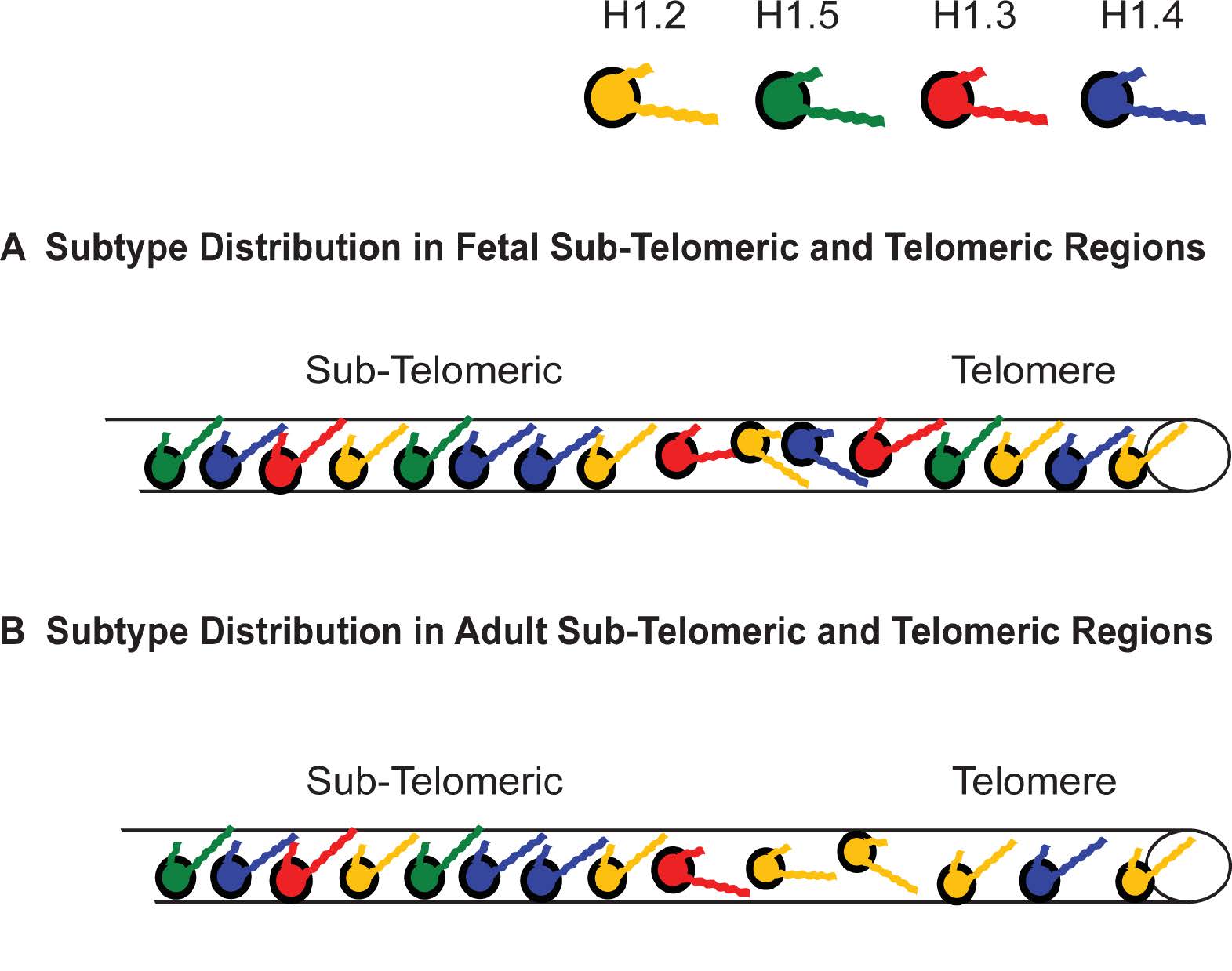
    [14] Parseghian MH, Newcomb RL, Winokur ST, et al. (2000) The distribution of somatic H1 subtypes is non-random on active vs. inactive chromatin: Distribution in human fetal fibroblasts. Chromosome Res 8: 405-424.
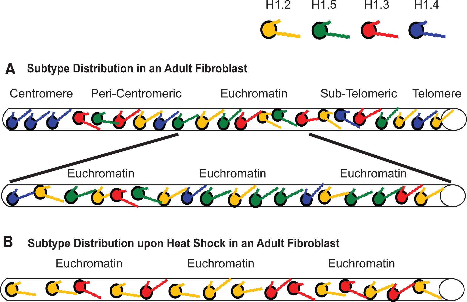
    [15] Parseghian MH, Newcomb RL, Hamkalo BA (2001) The distribution of somatic H1 subtypes is non-random on active vs. inactive chromatin II: Distribution in human adult fibroblasts. J Cell Biochem 83: 643-659.
    [16] Eick S, Nicolai M, Mumberg D, et al. (1989) Human H1 histones: Conserved and varied sequence elements in two H1 subtype genes. Eur J Cell Bio 49: 110-115.
    [17] Albig W, Kardalinou E, Drabent B, et al. (1991) Isolation and characterization of two human H1 histone genes within clusters of core histone genes. Genomics 10: 940-948. doi: 10.1016/0888-7543(91)90183-F
    [18] Albig W, Meergans T, Doenecke D (1997) Characterization of the H1.5 gene completes the set of human H1 subtype genes. Gene 184: 141-148.
    [19] Bustin M, Cole RD (1968) Species and organ specificity in very lysine-rich histones. J Biol Chem 243: 4500-4505.
    [20] Bustin M, Cole RD (1969) A study of the multiplicity of lysine-rich histones. J Biol Chem 244: 5286-5290.
    [21] Bradbury EM, Crane-Robinson C, Johns EW (1972) Specific conformations and interactions in chicken erythrocyte histone F2C. Nat New Biol 238: 262-264. doi: 10.1038/newbio238262a0
    [22] Smith BJ, Walker JM, Johns EW (1980) Structural homology between a mammalian H1(0) subfraction and avian erythrocyte-specific histone H5. FEBS Lett 112: 42-44. doi: 10.1016/0014-5793(80)80122-0
    [23] Seyedin SM, Kistler WS (1979) H1 histone subfractions of mammalian testes. 1. Organ specificity in the rat. Biochemistry 18: 1371-1375.
    [24] Seyedin SM, Kistler WS (1979) H1 histone subfractions of mammalian testes. 2. Organ specificity in mice and rabbits. Biochemistry 18: 1376-1379.
    [25] Seyedin SM, Kistler WS (1980) Isolation and characterization of rat testis H1t: an H1 histone variant associated with spermatogenesis. J Biol Chem 255: 5949-5954.
    [26] Yamamoto T, Horikoshi M (1996) Cloning of the cDNA encoding a novel subtype of histone H1. Gene 173: 281-285. doi: 10.1016/0378-1119(96)00020-0
    [27] Tanaka M, Hennebold JD, Macfarlane J, et al. (2001) A mammalian oocyte-specific linker histone gene H1oo: Homology with the genes for the oocyte-specific cleavage stage histone (cs-H1) of sea urchin and the B4/H1M histone of the frog. Development 128: 655-664.
    [28] Yan W, Ma L, Burns KH, et al. (2003) HILS1 is a spermatid-specific linker histone H1-like protein implicated in chromatin remodeling during mammalian spermiogenesis. Proc Natl Acad Sci U S A 100: 10546-10551. doi: 10.1073/pnas.1837812100
    [29] Martianov I, Brancorsini S, Catena R, et al. (2005) Polar nuclear localization of H1T2, a histone H1 variant, required for spermatid elongation and DNA condensation during spermiogenesis. Proc Natl Acad Sci U S A 102: 2808-2813. doi: 10.1073/pnas.0406060102
    [30] Parseghian MH, Henschen AH, Krieglstein KG, et al. (1994) A proposal for a coherent mammalian histone H1 nomenclature correlated with amino acid sequences. Protein Sci 3: 575-587.
    [31] Schlissel MS, Brown DD (1984) The transcriptional regulation of Xenopus 5S RNA genes in chromatin: The roles of active stable transcription complexes and histone H1. Cell 37: 903-913. doi: 10.1016/0092-8674(84)90425-2
    [32] Shimamura A, Sapp M, Rodriguez-Campos A, et al. (1989) Histone H1 represses transcription from minichromosomes assembled in vitro. Mol Cell Biol 9: 5573-5584. doi: 10.1128/MCB.9.12.5573
    [33] Lu ZH, Sittman DB, Romanowski P, et al. (1998) Histone H1 reduces the frequency of initiation in Xenopus egg extract by limiting the assembly of prereplication complexes on sperm chromatin. Molec Bio Cell 9: 1163-1176. doi: 10.1091/mbc.9.5.1163
    [34] Laybourn PJ, Kadonaga JT (1991) Role of nucleosomal cores and histone H1 in regulation of transcription by RNA polymerase II. Science 254: 238-245. doi: 10.1126/science.1718039
    [35] Lu ZH, Xu H, Leno GH (1999) DNA replication in quiescent cell nuclei: Regulation by the nuclear envelope and chromatin structure. Molec Bio Cell 10: 4091-4106. doi: 10.1091/mbc.10.12.4091
    [36] Carruthers LM, Bednar J, Woodcock CL, et al. (1998) Linker histones stabilize the intrinsic salt-dependent folding of nucleosomal arrays: Mechanistic ramifications for higher-order chromatin folding. Biochemistry 37: 14776-14787. doi: 10.1021/bi981684e
    [37] Parseghian MH, Luhrs KA (2006) Beyond the Walls of the Nucleus: The Role of Histones in Cellular Signaling and Innate Immunity. Biochem Cell Biol 84: 589-604. doi: 10.1139/o06-082
    [38] 
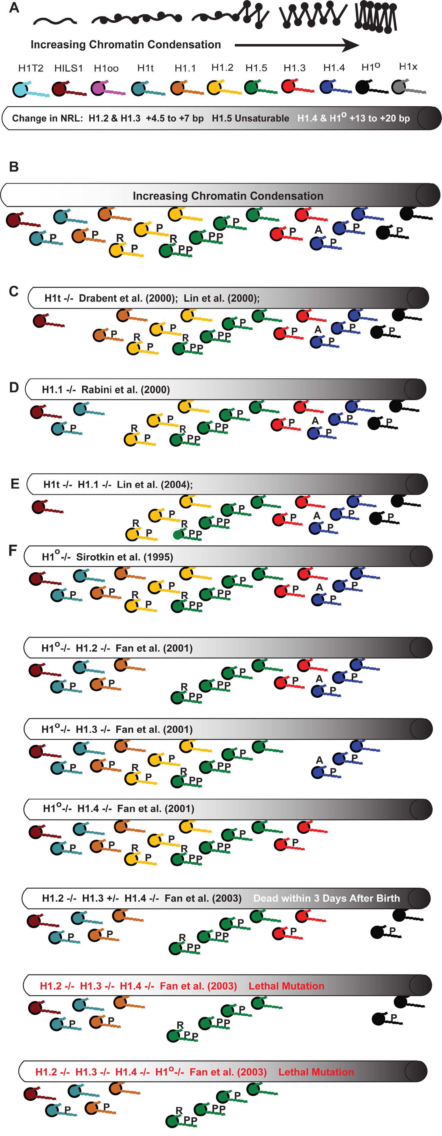
Sirotkin AM, Edelmann W, Cheng G, et al. (1995) Mice develop normally without the H1° linker histone. Proc Natl Acad Sci U S A 92: 6434-6438. doi: 10.1073/pnas.92.14.6434
    [39] Lin Q, Sirotkin AM, Skoultchi AI (2000) Normal spermatogenesis in mice lacking the testis-specific linker histone H1t. Mol Cell Biol 20: 2122-2128. doi: 10.1128/MCB.20.6.2122-2128.2000
    [40] Fan Y, Sirotkin AM, Russell RG, et al. (2001) Individual somatic H1 subtypes are dispensable for mouse development even in mice lacking the H1° replacement subtype. Mol Cell Biol 21: 7933-7943. doi: 10.1128/MCB.21.23.7933-7943.2001
    [41] Allan J, Hartman PG, Crane-Robinson C, et al. (1980) The structure of histone H1 and its location in chromatin. Nature 288: 675-679. doi: 10.1038/288675a0
    [42] Hartman PG, Chapman GE, MossT, et al. (1977) Studies on the role and mode of operation of the very-lysine-rich histone H1 in eukaryote chromatin. Eur J Biochem 77: 45-51. doi: 10.1111/j.1432-1033.1977.tb11639.x
    [43] Izzo A, Kamieniarz K, Schneider R (2008) The histone H1 family: specific members, specific functions? Biol Chem 389: 333-343.
    [44] Ramakrishnan V, Finch JT, Graziano V, et al. (1993) Crystal structure of globular domain of histone H5 and its implications for nucleosome binding. Nature 362: 219-223. doi: 10.1038/362219a0
    [45] Cerf C, Lippens G, Muyldermans S, et al. (1993) Homo- and heteronuclear two-dimensional NMR studies of the globular domain of histone H1: sequential assignment and secondary structure. Biochemistry 32: 11345-11351. doi: 10.1021/bi00093a011
    [46] Zhou BR, Feng H, Kato H, et al. (2013) Structural insights into the histone H1-nucleosome complex. Proc Natl Acad Sci U S A 110: 19390-19395. doi: 10.1073/pnas.1314905110
    [47] Zhou BR, Jiang J, Feng H, et al. (2015) Structural Mechanisms of Nucleosome Recognition by Linker Histones. Mol Cell 59: 628-638. doi: 10.1016/j.molcel.2015.06.025
    [48] Syed SH, Goutte-Gattat D, Becker N, et al. (2010) Single-base resolution mapping of H1-nucleosome interactions and 3D organization of the nucleosome. Proc Natl Acad Sci U S A 107: 9620-9625. doi: 10.1073/pnas.1000309107
    [49] Fan L, Roberts VA (2006) Complex of linker histone H5 with the nucleosome and its implications for chromatin packing. Proc Natl Acad Sci U S A 103: 8384-8389.
    [50] An W, Leuba SH, van Holde KE, et al. (1998) Linker histone protects linker DNA on only one side of the core particle and in a sequence-dependent manner. Proc Natl Acad Sci U S A 95: 3396-3401. doi: 10.1073/pnas.95.7.3396
    [51] Thomas JO (1999) Histone H1: Location and role. Curr Opin Cell Biol 11: 312-317. doi: 10.1016/S0955-0674(99)80042-8
    [52] Brown DT, Izard T, Misteli T (2006) Mapping the interaction surface of linker histone H1(0) with the nucleosome of native chromatin in vivo. Nat Struct Mol Biol 13: 250-255. doi: 10.1038/nsmb1050
    [53] Song F, Chen P, Sun D, et al. (2014) Cryo-EM study of the chromatin fiber reveals a double helix twisted by tetranucleosomal units. Science 344: 376-380. doi: 10.1126/science.1251413
    [54] George EM, Izard T, Anderson SD, et al. (2010) Nucleosome interaction surface of linker histone H1c is distinct from that of H1(0). J Biol Chem 285: 20891-20896. doi: 10.1074/jbc.M110.108639
    [55] Vila R, Ponte I, Collado M, et al. (2001) DNA-induced a-helical structure in the NH2 -terminal domain of histone H1. J Biol Chem 276: 46429-46435. doi: 10.1074/jbc.M106952200
    [56] Vila R, Ponte I, Jiménez MA, et al. (2002) An inducible helix Gly-Gly helix motif in the N-terminal domain of histone H1e: A CD and NMR study. Protein Sci 11: 214-220.
    [57] Becker M, Becker A, Miyara F, et al. (2005) Differential in vivo binding dynamics of somatic and oocyte-specific linker histones in oocytes and during ES cell nuclear transfer. Mol Biol Cell 16: 3887-3895. doi: 10.1091/mbc.E05-04-0350
    [58] Vyas P, Brown DT (2012) N- and C-terminal domains determine differential nucleosomal binding geometry and affinity of linker histone isotypes H1(0) and H1c. J Biol Chem 287: 11778-11787. doi: 10.1074/jbc.M111.312819
    [59] Kalashnikova AA, Winkler DD, McBryant SJ, et al. (2013) Linker histone H1.0 interacts with an extensive network of proteins found in the nucleolus. Nucleic Acids Res 41: 4026-4035.
    [60] Caterino TL, Hayes JJ (2011) Structure of the H1 C-terminal domain and function in chromatin condensation. Biochem Cell Biol 89: 35-44. doi: 10.1139/O10-024
    [61] Hill CS, Martin SR, Thomas JO (1989) A stable a-helical element in the carboxy-terminal domain of free and chromatin-bound histone H1 from sea urchin sperm. EMBO J 8: 2591-2599.
    [62] Vila R, Ponte I, Jiménez MA, et al. (2000) A helix-turn motif in the C-terminal domain of histone H1. Protein Sci 9: 627-636.
    [63] Vila R, Ponte I, Collado M, et al. (2001) Induction of secondary structure in a COOH-terminal peptide of histone H1 by interaction with the DNA. J Biol Chem 276: 30898-30903. doi: 10.1074/jbc.M104189200
    [64] Roque A, Iloro I, Ponte I, et al. (2005) DNA-induced secondary structure of the carboxyl-terminal domain of histone H1. J Biol Chem 280: 32141-32147. doi: 10.1074/jbc.M505636200
    [65] Hendzel MJ, Lever MA, Crawford E, et al. (2004) The C-terminal domain is the primary determinant of histone H1 binding to chromatin in vivo. J Biol Chem 279: 20028-20034. doi: 10.1074/jbc.M400070200
    [66] Clausell J, Happel N, Hale TK, et al. (2009) Histone H1 subtypes differentially modulate chromatin condensation without preventing ATP-dependent remodeling by SWI/SNF or NURF. PLoS ONE 4: e0007243.
    [67] Lu X, Hansen JC (2004) Identification of specific functional subdomains within the linker histone H1° C-terminal domain. J Biol Chem 279: 8701-8707. doi: 10.1074/jbc.M311348200
    [68] De S, Brown DT, Lu ZH, et al. (2002) Histone H1 variants differentially inhibit DNA replication through an affinity for chromatin mediated by their carboxyl-terminal domains. Gene 292: 173-181. doi: 10.1016/S0378-1119(02)00675-3
    [69] Hansen JC, Lu X, Ross ED, et al. (2006) Intrinsic protein disorder, amino acid composition, and histone terminal domains. J Biol Chem 281: 1853-1856. doi: 10.1074/jbc.R500022200
    [70] Finn RM, Ellard K, Eirin-Lopez JM, et al. (2012) Vertebrate nucleoplasmin and NASP: egg histone storage proteins with multiple chaperone activities. FASEB J 26: 4788-4804. doi: 10.1096/fj.12-216663
    [71] Karetsou Z, Sandaltzopoulos R, Frangou-Lazaridis M, et al. (1998) Prothymosin a modulates the interaction of histone H1 with chromatin. Nucl Acids Res 26: 3111-3118. doi: 10.1093/nar/26.13.3111
    [72] Lu X, Hamkalo BA, Parseghian MH, et al. (2009) Chromatin condensing functions of the linker histone C-terminal domain are mediated by specific amino acid composition and intrinsic protein disorder. Biochemistry 48: 164-172. doi: 10.1021/bi801636y
    [73] Widlak P, Kalinowska M, Parseghian MH, et al. (2005) The histone H1 C-terminal domain binds to the apoptotic nuclease, DNA Fragmentation Factor (DFF40/CAD) and stimulates DNA cleavage. Biochemistry 44: 7871-7878. doi: 10.1021/bi050100n
    [74] Roque A, Orrego M, Ponte I, et al. (2004) The preferential binding of histone H1 to DNA scaffold-associated regions is determined by its C-terminal domain. Nucleic Acids Res 32: 6111-6119. doi: 10.1093/nar/gkh945
    [75] Stasevich TJ, Mueller F, Brown DT, et al. (2010) Dissecting the binding mechanism of the linker histone in live cells: an integrated FRAP analysis. EMBO J 29: 1225-1234. doi: 10.1038/emboj.2010.24
    [76] Wisniewski JR, Zougman A, Kruger S, et al. (2007) Mass spectrometric mapping of linker histone H1 variants reveals multiple acetylations, methylations, and phosphorylation as well as differences between cell culture and tissue. Mol Cell Proteomics 6: 72-87.
    [77] Ajiro K, Shibata K, Nishikawa Y (1990) Subtype-specific cyclic AMP-dependent histone H1 phosphorylation at the differentiation of mouse neuroblastoma cells. J Biol Chem 265: 6494-6500.
    [78] Hill CS, Rimmer JM, Green BN, et al. (1991) Histone-DNA interactions and their modulation by phosphorylation of Ser-Pro-X-Lys/Arg motifs. EMBO J 10: 1939-1948.
    [79] Sarg B, Helliger W, Talasz H, et al. (2006) Histone H1 phosphorylation occurs site-specifically during interphase and mitosis: identification of a novel phosphorylation site on histone H1. J Biol Chem 281: 6573-6580. doi: 10.1074/jbc.M508957200
    [80] Suzuki M (1989) SPKK, a new nucleic acid-binding unit of protein found in histone. EMBO J 8: 797-804.
    [81] Lopez R, Sarg B, Lindner H, et al. (2015) Linker histone partial phosphorylation: effects on secondary structure and chromatin condensation. Nucleic Acids Res 43: 4463-4476. doi: 10.1093/nar/gkv304
    [82] Talasz H, Helliger W, Puschendorf B, et al. (1996) In vivo phosphorylation of histone H1 variants during the cell cycle. Biochemistry 35: 1761-1767. doi: 10.1021/bi951914e
    [83] Riquelme PT, Burzio LO, Koide SS (1979) ADP ribosylation of rat liver lysine-rich histone in vitro. J Biol Chem 254: 3018-3028.
    [84] D'Erme M, Zardo G, Reale A, et al. (1996) Co-operative interactions of oligonucleosomal DNA with the H1e histone variant and its poly(ADP-ribosyl)ated isoform. Biochem J 316: 475-480. doi: 10.1042/bj3160475
    [85] de Murcia G, Huletsky A, Lamarre D, et al. (1986) Modulation of chromatin superstructure induced by poly(ADP-ribose) synthesis and degradation. J Biol Chem 261: 7011-7017.
    [86] Vaquero A, Scher M, Lee D, et al. (2004) Human SirT1 interacts with histone H1 and promotes formation of facultative heterochromatin. Mol Cell 16: 93-105. doi: 10.1016/j.molcel.2004.08.031
    [87] Kuzmichev A, Jenuwein T, Tempst P, et al. (2004) Different Ezh2-containing complexes target methylation of histone H1 or nucleosomal histone H3. Molec Cell 14: 183-193. doi: 10.1016/S1097-2765(04)00185-6
    [88] Weiss T, Hergeth S, Zeissler U, et al. (2010) Histone H1 variant-specific lysine methylation by G9a/KMT1C and Glp1/KMT1D. Epigenetics Chromatin 3: 7. doi: 10.1186/1756-8935-3-7
    [89] Th'ng JPH, Sung R, Ye M, et al. (2005) H1 family histones in the nucleus: Control of binding and localization by the C-terminal domain. J Biol Chem 280: 27809-27814. doi: 10.1074/jbc.M501627200
    [90] Izzo A, Kamieniarz-Gdula K, Ramirez F, et al. (2013) The genomic landscape of the somatic linker histone subtypes H1.1 to H1.5 in human cells. Cell Rep 3: 2142-2154.
    [91] Cao K, Lailler N, Zhang Y, et al. (2013) High-resolution mapping of h1 linker histone variants in embryonic stem cells. PLoS Genet. 9: e1003417. doi: 10.1371/journal.pgen.1003417
    [92] Appels R, Bolund L, Ringertz NR (1974) Biochemical analysis of reactivated chick erythrocyte nuclei isolated from chick/HeLa heterokaryons. J Mol Biol 87: 339-355. doi: 10.1016/0022-2836(74)90154-5
    [93] 
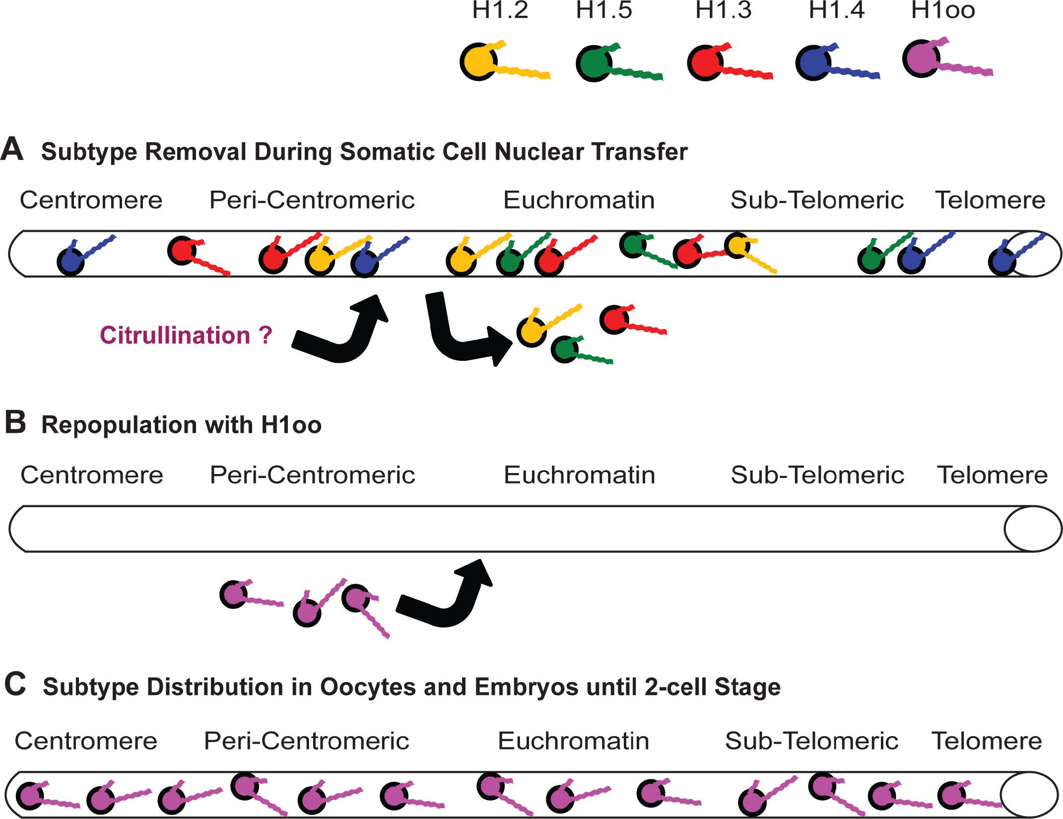
Gao S, Chung YG, Parseghian MH, et al. (2004) Rapid H1 linker histone transitions following fertilization or somatic cell nuclear transfer: evidence for a uniform developmental program in mice. Dev Biol 266: 62-75. doi: 10.1016/j.ydbio.2003.10.003
    [94] Dimitrov S, Wolffe AP (1996) Remodeling somatic nuclei in Xenopus laevis egg extracts: molecular mechanisms for the selective release of histones H1 and H1° from chromatin and the acquisition of transcriptional competence. EMBO J 15: 5897-5906.
    [95] Teranishi T, Tanaka M, Kimoto S, et al. (2004) Rapid replacement of somatic linker histones with the oocyte-specific linker histone H1foo in nuclear transfer. Dev Biol 266: 76-86. doi: 10.1016/j.ydbio.2003.10.004
    [96] Misteli T, Gunjan A, Hock R, et al. (2000) Dynamic binding of histone H1 to chromatin in living cells. Nature 408: 877-881. doi: 10.1038/35048610
    [97] Phair RD, Scaffidi P, Elbi C, et al. (2004) Global nature of dynamic protein-chromatin interactions in vivo: Three dimensional genome scanning and dynamic interaction networks of chromatin proteins. Mol Cell Biol 24: 6393-6402. doi: 10.1128/MCB.24.14.6393-6402.2004
    [98] Bustin M, Catez F, Lim J-H (2005) The dynamics of histone H1 function in chromatin. Molec Cell 17: 617-620. doi: 10.1016/j.molcel.2005.02.019
    [99] Raghuram N, Carrero G, Stasevich TJ, et al. (2010) Core histone hyperacetylation impacts cooperative behavior and high-affinity binding of histone H1 to chromatin. Biochemistry 49: 4420-4431. doi: 10.1021/bi100296z
    [100] Kimura H, Cook PR (2001) Kinetics of core histones in living human cells: Little exchange of H3 and H4 and some rapid exchange of H2B. J Cell Biology 153: 1341-1353. doi: 10.1083/jcb.153.7.1341
    [101] Contreras A, Hale TK, Stenoien DL, et al. (2003) The dynamic mobility of histone H1 is regulated by Cyclin/CDK Phosphorylation. Mol Cell Biol 23: 8626-8636. doi: 10.1128/MCB.23.23.8626-8636.2003
    [102] Yellajoshyula D, Brown DT (2006) Global modulation of chromatin dynamics mediated by dephosphorylation of linker histone H1 is necessary for erythroid differentiation. Proc Natl Acad Sci U S A 103: 18568-18573. doi: 10.1073/pnas.0606478103
    [103] Takata H, Matsunaga S, Morimoto A, et al. (2007) H1.X with different properties from other linker histones is required for mitotic progression. FEBS Lett 581: 3783-3788.
    [104] Lever MA, Th'ng JPH, Sun X, et al. (2000) Rapid exchange of histone H1.1 on chromatin in living human cells. Nature 408: 873-876.
    [105] Christophorou MA, Castelo-Branco G, Halley-Stott RP, et al. (2014) Citrullination regulates pluripotency and histone H1 binding to chromatin. Nature 507: 104-108. doi: 10.1038/nature12942
    [106] Liao LW, Cole RD (1981) Condensation of dinucleosomes by individual subfractions of H1 histone. J Biol Chem 256: 10124-10128.
    [107] Khadake JR, Rao MR (1995) DNA- and chromatin-condensing properties of rat testes H1a and H1t compared to those of rat liver H1bdec; H1t is a poor condenser of chromatin. Biochemistry 34: 15792-15801. doi: 10.1021/bi00048a025
    [108] Talasz H, Sapojnikova N, Helliger W, et al. (1998) In vitro binding of H1 histone subtypes to nucleosomal organized mouse mammary tumor virus long terminal repeat promotor. J Biol Chem 273: 32236-32243. doi: 10.1074/jbc.273.48.32236
    [109] Hannon R, Bateman E, Allan J, et al. (1984) Control of RNA polymerase binding to chromatin by variations in linker histone composition. J Mol Biol 180: 131-149. doi: 10.1016/0022-2836(84)90434-0
    [110] Orrego M, Ponte I, Roque A, et al. (2007) Differential affinity of mammalian histone H1 somatic subtypes for DNA and chromatin. BMC Biol 5: 22. doi: 10.1186/1741-7007-5-22
    [111] Brown DT, Alexander BT, Sittman DB (1996) Differential effect of H1 variant overexpression on cell cycle progression and gene expression. Nucl Acids Res 24: 486-493. doi: 10.1093/nar/24.3.486
    [112] Bhan S, May W, Warren SL, et al. (2008) Global gene expression analysis reveals specific and redundant roles for H1 variants, H1c and H1(0), in gene expression regulation. Gene 414: 10-18. doi: 10.1016/j.gene.2008.01.025
    [113] Funayama R, Saito M, Tanobe H, et al. (2006) Loss of linker histone H1 in cellular senescence. J. Cell Biol 175: 869-880. doi: 10.1083/jcb.200604005
    [114] Kasinsky HE, Lewis JD, Dacks JB, et al. (2001) Origin of H1 linker histones. FASEB J 15: 34-42. doi: 10.1096/fj.00-0237rev
    [115] Wu M, Allis CD, Richman R, et al. (1986) An intervening sequence in an unusual histone H1 gene of Tetrahymena thermophila. Proc Natl Acad Sci U S A 83: 8674-8678. doi: 10.1073/pnas.83.22.8674
    [116] Schulze E, Schulze B (1995) The vertebrate linker histones H1°, H5 and H1M are descendants of invertebrate ""orphon"" histone H1 genes. J Mol Evol 41: 833-840.
    [117] Ponte I, Vidal-Taboada JM, Suau P (1998) Evolution of the vertebrate H1 histone class: Evidence for the functional differentiation of the subtypes. Mol Biol Evol 15: 702-708. doi: 10.1093/oxfordjournals.molbev.a025973
    [118] Downs JA, Kosmidou E, Morgan A, et al. (2003) Suppression of homologous recombination by the Saccharomyces cerevisiae linker histone. Molec Cell 11: 1685-1692. doi: 10.1016/S1097-2765(03)00197-7
    [119] Hellauer K, Sirard E, Turcotte B (2001) Decreased expression of specific genes in yeast cells lacking histone H1. J Biol Chem 276: 13587-13592.
    [120] Shen X, Gorovsky MA (1996) Linker histone H1 regulates specific gene expression but not global transcription in vivo. Cell 86: 475-483. doi: 10.1016/S0092-8674(00)80120-8
    [121] Nalabothula N, McVicker G, Maiorano J, et al. (2014) The chromatin architectural proteins HMGD1 and H1 bind reciprocally and have opposite effects on chromatin structure and gene regulation. BMC. Genomics. 15, 92.
    [122] Meergans T, Albig W, Doenecke D (1997) Varied expression patterns of human H1 histone genes in different cell lines. DNA Cell Biol 16: 1041-1049. doi: 10.1089/dna.1997.16.1041
    [123] Pina B, Martinez P, Suau P (1987) Changes in H1 complement in differentiating rat-brain cortical neurons. Eur J Biochem 164: 71-76. doi: 10.1111/j.1432-1033.1987.tb10994.x
    [124] Kamieniarz K, Izzo A, Dundr M, et al. (2012) A dual role of linker histone H1.4 Lys 34 acetylation in transcriptional activation. Genes Dev 26: 797-802.
    [125] Huang H-C, Cole RD (1984) The distribution of H1 histone is nonuniform in chromatin and correlates with different degrees of condensation. J Biol Chem 259: 14237-14242.
    [126] Gunjan A, Alexander BT, Sittman DB, et al. (1999) Effects of H1 histone variant overexpression on chromatin structure. J Biol Chem 274: 37950-37956. doi: 10.1074/jbc.274.53.37950
    [127] Krishnakumar R, Gamble MJ, Frizzell KM, et al. (2008) Reciprocal binding of PARP-1 and histone H1 at promoters specifies transcriptional outcomes. Science. 319: 819-821. doi: 10.1126/science.1149250
    [128] Parseghian MH, Harris DA, Rishwain DR, et al. (1994) Characterization of a set of antibodies specific for three human histone H1 subtypes. Chromosoma 103: 198-208. doi: 10.1007/BF00368013
    [129] Boulikas T, Bastin B, Boulikas P, et al. (1990) Increase in histone poly(ADP-ribosylation) in mitogen-activated lymphoid cells. Exp Cell Res 187: 77-84. doi: 10.1016/0014-4827(90)90119-U
    [130] Parseghian MH, Henschen AH, Krieglstein KG, et al. (1994) A proposal for a coherent mammalian histone H1 nomenclature correlated with amino acid sequences. Protein Sci 3: 575-587.
    [131] Higurashi M, Adachi H, Ohba Y (1987) Synthesis and degradation of H1 histone subtypes in mouse lymphoma L5178Y cells. J Biol Chem 262: 13075-13080.
    [132] Cheng G, Nandi A, Clerk S, et al. (1989) Different 3'-end processing produces two independently regulated mRNAs from a single H1 histone gene. Proc Natl Acad Sci U S A 86: 7002-7006. doi: 10.1073/pnas.86.18.7002
    [133] Routh A, Sandin S, Rhodes D (2008) Nucleosome repeat length and linker histone stoichiometry determine chromatin fiber structure. Proc Natl Acad Sci U S A 105: 8872-8877. doi: 10.1073/pnas.0802336105
    [134] Beshnova DA, Cherstvy AG, Vainshtein Y, et al. (2014) Regulation of the nucleosome repeat length in vivo by the DNA sequence, protein concentrations and long-range interactions. PLoS Comput Biol 10: e1003698. doi: 10.1371/journal.pcbi.1003698
    [135] Chadee DN, Taylor WR, Hurta RAR, et al. (1995) Increased phosphorylation of histone H1 in mouse fibroblasts transformed with oncogenes or constitutively active mitogen-activated protein kinase kinase. J Biol Chem 270: 20098-20105. doi: 10.1074/jbc.270.34.20098
    [136] Chadee DN, Allis CD, Wright JA, et al. (1997) Histone H1b phosphorylation is dependent upon ongoing transcription and replication in normal and ras-transformed mouse fibroblasts. J Biol Chem 272: 8113-8116. doi: 10.1074/jbc.272.13.8113
    [137] Li JY, Patterson M, Mikkola HK, et al. (2012) Dynamic distribution of linker histone H1.5 in cellular differentiation. PLoS Genet. 8: e1002879.
    [138] Lee H, Habas R, Abate-Shen C (2004) Msx1 cooperates with histone H1b for inhibition of transcription and myogenesis. Science 304: 1675-1678. doi: 10.1126/science.1098096
    [139] Wang X, Peng Y, Ma Y, et al. (2004) Histone H1-like protein participates in endothelial cell-specific activation of the von Willebrand factor promoter. Blood 104: 1725-1732. doi: 10.1182/blood-2004-01-0082
    [140] Kaludov NK, Pabon-Pena L, Seavy M, et al. (1997) A mouse histone H1 variant, H1b, binds preferentially to a regulatory sequence within a mouse H3.2 replication-dependent histone gene. J Biol Chem 272: 15120-15127.
    [141] Oberg C, Izzo A, Schneider R, et al. (2012) Linker histone subtypes differ in their effect on nucleosomal spacing in vivo. J Mol Biol 419: 183-197. doi: 10.1016/j.jmb.2012.03.007
    [142] Pehrson JR, Cole RD (1982) Histone H1 subfractions and H1° turnover at different rates in nondividing cells. Biochemistry 21: 456-460. doi: 10.1021/bi00532a006
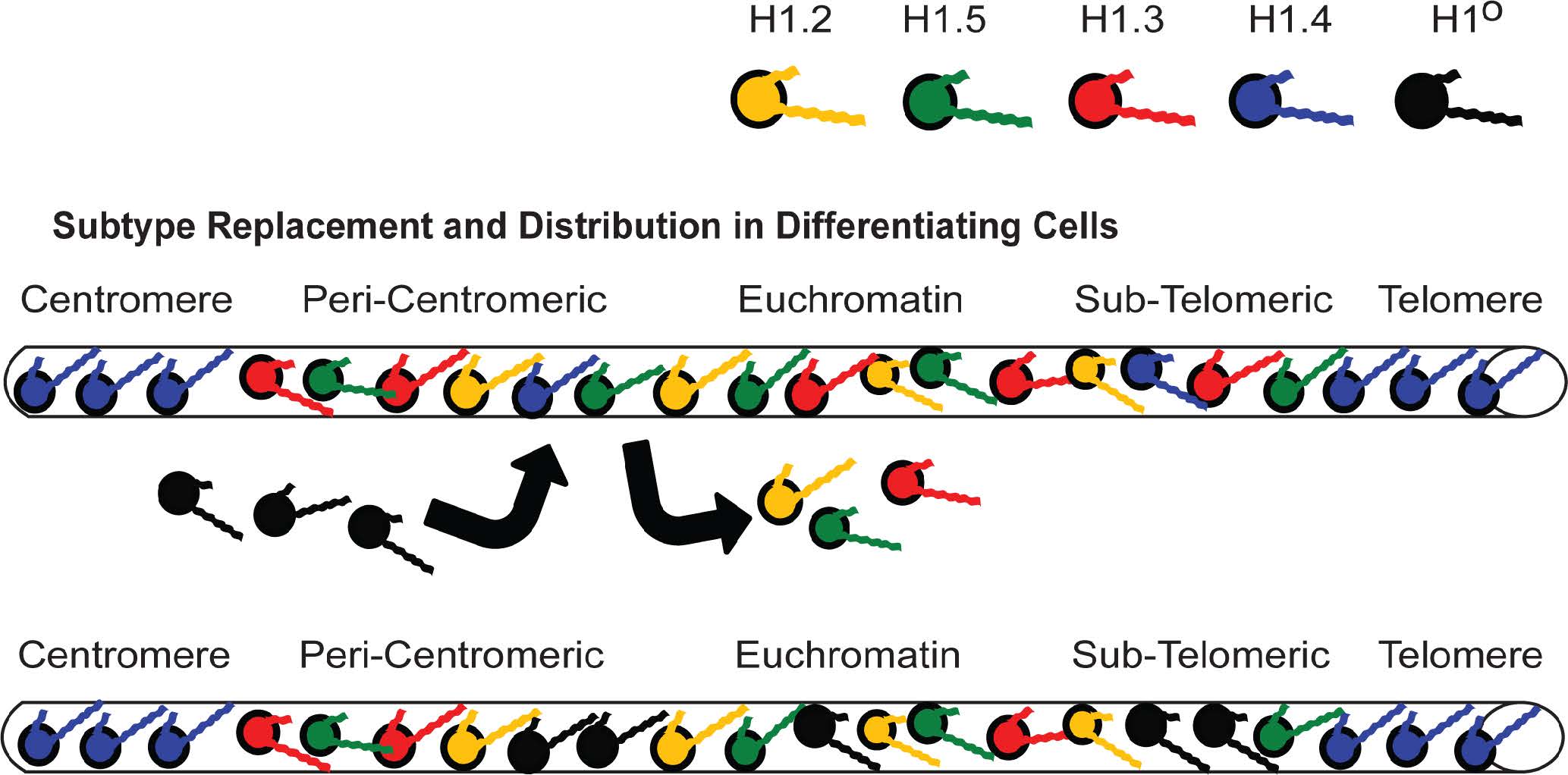
    [143] Zlatanova JS, Doenecke D (1994) Histone H1°: A major player in cell differentiation? FASEB J 8: 1260-1268.
    [144] Gabrilovich DI, Cheng P, Fan Y, et al. (2002) H1(0) histone and differentiation of dendritic cells. A molecular target for tumor-derived factors. J Leukoc Biol 72: 285-296.
    [145] Lennox RW, Cohen LH (1983) The histone H1 complements of dividing and nondividing cells of the mouse. J Biol Chem 258: 262-268.
    [146] Rasheed BKA, Whisenant EC, Ghai RD, et al. (1989) Biochemical and immunocytochemical analysis of a histone H1 variant from the mouse testis. J Cell Sci 94: 61-71.
    [147] Franke K, Drabent B, Doenecke D (1998) Expression of murine H1 histone genes during postnatal development. Biochim Biophys Acta 1398: 232-242. doi: 10.1016/S0167-4781(98)00062-1
    [148] Lennox RW (1984) Differences in evolutionary stability among mammalian H1 subtypes: Implications for the roles of H1 subtypes in chromatin. J Biol Chem 259: 669-672.
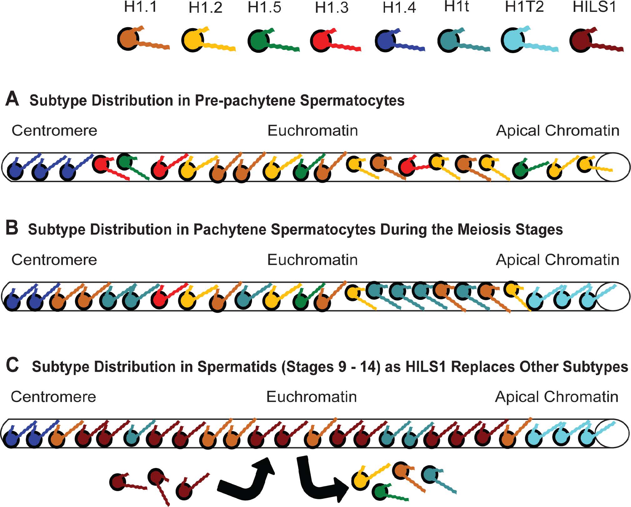
    [149] Lennox RW, Cohen LH (1984) The alterations in H1 histone complement during mouse spermatogenesis and their significance for H1 subtype function. Dev Biol 103, 80-84.
    [150] Rabini S, Franke K, Saftig P, et al. (2000) Spermatogenesis in mice is not affected by histone H1.1 deficiency. Exp Cell Res 255: 114-124. doi: 10.1006/excr.1999.4767
    [151] Oko RJ, Jando V, Wagner CL, et al. (1996) Chromatin reorganization in rat spermatids during the disappearance of testis-specific histone, H1t, and the appearance of transition proteins TP1 and TP2. Biol Reprod 54: 1141-1157. doi: 10.1095/biolreprod54.5.1141
    [152] de Lucia F, Faraone-Mennella MR, D'Erme M, et al. (1994) Histone-induced condensation of rat testis chromatin: Testis-specific H1t versus somatic H1 variants. Biochem Biophys Res Commun 198: 32-39. doi: 10.1006/bbrc.1994.1005
    [153] Catena R, Ronfani L, Sassone-Corsi P, et al. (2006) Changes in intranuclear chromatin architecture induce bipolar nuclear localization of histone variant H1T2 in male haploid spermatids. Dev Biol 296: 231-238. doi: 10.1016/j.ydbio.2006.04.458
    [154] Tanaka H, Iguchi N, Isotani A, et al. (2005) HANP1/H1T2, a novel histone H1-like protein involved in nuclear formation and sperm fertility. Mol Cell Biol 25: 7107-7119. doi: 10.1128/MCB.25.16.7107-7119.2005
    [155] Saeki H, Ohsumi K, Aihara H, et al. (2005) Linker histone variants control chromatin dynamics during early embryogenesis. Proc Natl Acad Sci U S A 102: 5697-5702. doi: 10.1073/pnas.0409824102
    [156] Tanaka M, Kihara M, Hennebold JD, et al. (2005) H1FOO is coupled to the initiation of oocytic growth. Biol Reprod 72: 135-142. doi: 10.1095/biolreprod.104.032474
    [157] Nazarov IB, Shlyakhtenko LS, Lyubchenko YL, et al. (2008) Sperm chromatin released by nucleases. Syst Biol Reprod Med 54: 37-46. doi: 10.1080/19396360701876849
    [158] Sanchez-Vazquez ML, Flores-Alonso JC, Merchant-Larios H, et al. (2008) Presence and release of bovine sperm histone H1 during chromatin decondensation by heparin-glutathione. Syst Biol Reprod Med 54: 221-230. doi: 10.1080/19396360802357087
    [159] 
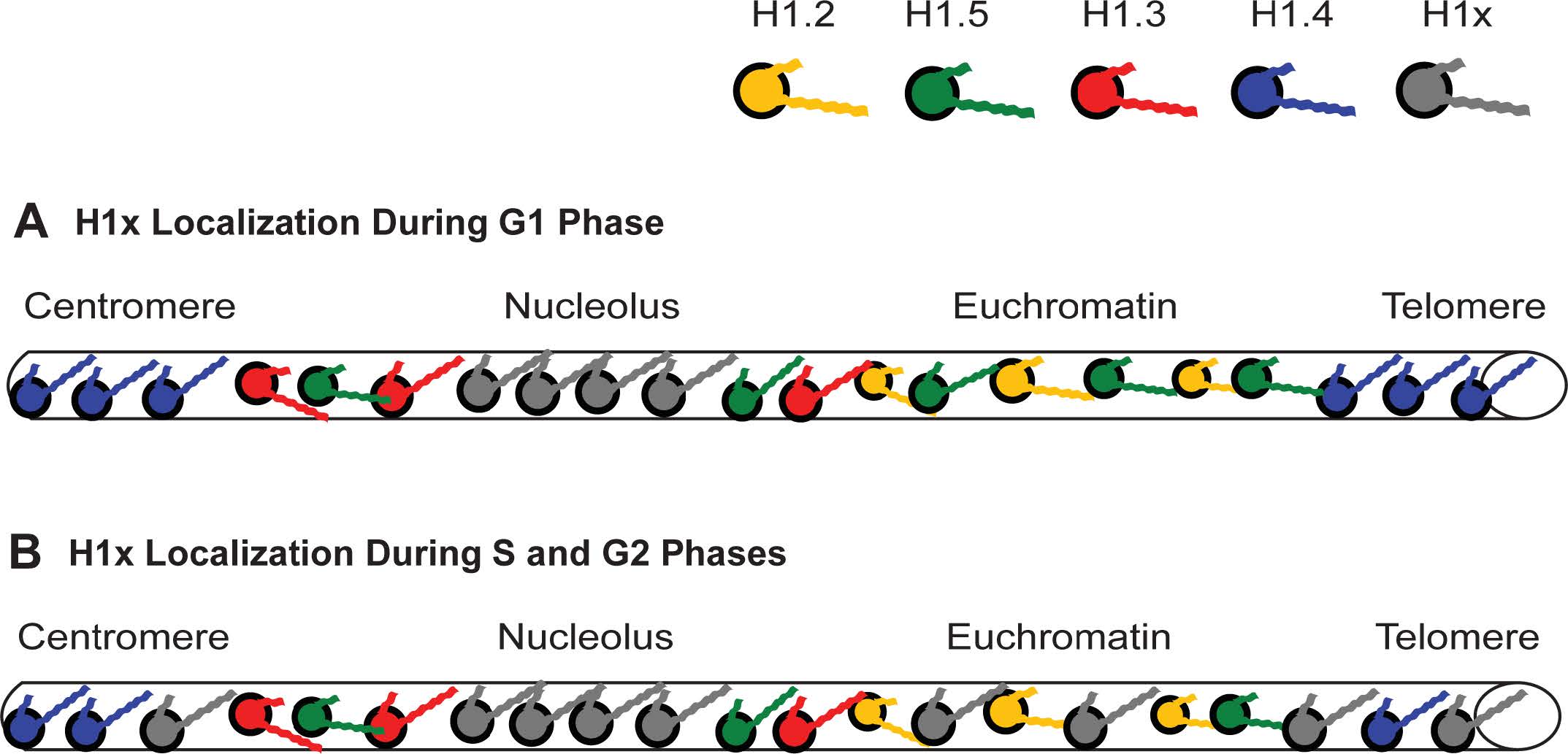
Stoldt S, Wenzel D, Schulze E, et al. (2007) G1 phase-dependent nucleolar accumulation of human histone H1x. Biol Cell 99: 541-552. doi: 10.1042/BC20060117
    [160] Mayor R, Izquierdo-Bouldstridge A, Millan-Arino L, et al. (2015) Genome distribution of replication-independent histone H1 variants shows H1.0 associated with nucleolar domains and H1X associated with RNA polymerase II-enriched regions. J Biol Chem 290: 7474-7491.
    [161] Happel N, Schulze E, Doenecke D (2005) Characterization of human histone H1x. Biol Chem 386: 541-551.
    [162] Drabent B, Saftig P, Bode C, et al. (2000) Spermatogenesis proceeds normally in mice without linker histone H1t. Histochem. Cell Biol 113: 433-442.
    [163] Drabent B, Benavente R, Hoyer-Fender S (2003) Histone H1t is not replaced by H1.1 or H1.2 in pachytene spermatocytes or spermatids of H1t-deficient mice. Cytogenet Genome Res 103: 307-313.
    [164] Lin Q, Inselman A, Han X, et al. (2004) Reductions in linker histone levels are tolerated in developing spermatocytes but cause changes in specific gene expression. J Biol Chem 279: 23525-23535. doi: 10.1074/jbc.M400925200
    [165] Fan Y, Nikitina T, Zhao J, et al. (2005) Histone H1 depletion in mammals alters global chromatin structure but causes specific changes in gene regulation. Cell 123: 1199-1212. doi: 10.1016/j.cell.2005.10.028
    [166] Zhang Y, Cooke M, Panjwani S, et al. (2012) Histone h1 depletion impairs embryonic stem cell differentiation. PLoS Genet 8: e1002691. doi: 10.1371/journal.pgen.1002691
    [167] Cherstvy AG, Teif VB (2014) Electrostatic effect of H1-histone protein binding on nucleosome repeat length. Phys Biol 11: 044001. doi: 10.1088/1478-3975/11/4/044001
    [168] Woodcock CL, Skoultchi AI, Fan Y (2006) Role of linker histone in chromatin structure and function: H1 stoichiometry and nucleosome repeat length. Chromosome Res 14: 17-25. doi: 10.1007/s10577-005-1024-3
    [169] Schiessel H (2003) The physics of chromatin. J Phys Condens Matter 15: R699-R774. doi: 10.1088/0953-8984/15/19/203
    [170] Bedoyan JK, Lejnine S, Makarov VL, et al. (1996) Condensation of rat telomere-specific nucleosomal arrays containing unusually short DNA repeats and histone H1. J Biol Chem 271: 18485-18493. doi: 10.1074/jbc.271.31.18485
    [171] Ascenzi R, Gantt JS (1999) Subnuclear distribution of the entire complement of linker histone variants in Arabidopsis thaliana. Chromosoma 108: 345-355. doi: 10.1007/s004120050386
    [172] O'Sullivan RJ, Karlseder J (2012) The great unravelling: chromatin as a modulator of the aging process. Trends Biochem Sci 37: 466-476. doi: 10.1016/j.tibs.2012.08.001
    [173] Oberdoerffer P, Michan S, McVay M, et al. (2008) SIRT1 redistribution on chromatin promotes genomic stability but alters gene expression during aging. Cell 135: 907-918. doi: 10.1016/j.cell.2008.10.025
    [174] O'Sullivan RJ, Kubicek S, Schreiber SL, et al. (2010) Reduced histone biosynthesis and chromatin changes arising from a damage signal at telomeres. Nat Struct Mol Biol 17: 1218-1225. doi: 10.1038/nsmb.1897
    [175] Feser J, Truong D, Das C, et al. (2010) Elevated histone expression promotes life span extension. Mol Cell 39: 724-735. doi: 10.1016/j.molcel.2010.08.015
    [176] Winokur ST, Bengtsson U, Feddersen J, et al. (1994) The DNA rearrangement associated with facioscapulohumeral muscular dystrophy involves a heterochromatin-associated repetitive element: Implications for a role of chromatin structure in the pathogenesis of the disease. Chromosome Res 2: 225-234. doi: 10.1007/BF01553323
    [177] Makarov VL, Lejnine S, Bedoyan JK, et al. (1993) Nucleosomal organization of telomere-specific chromatin in rat. Cell 73: 775-787. doi: 10.1016/0092-8674(93)90256-P
    [178] Pina B, Martinez P, Simon L, et al. (1984) Differential kinetics of histone H1° accumulation in neuronal and glial cells from rat cerebral cortex during postnatal development. Biochem Biophys Res Commun 123: 697-702. doi: 10.1016/0006-291X(84)90285-7
    [179] Drabent B, Kardalinou E, Doenecke D (1991) Structure and expression of the human testicular H1 histone (H1t) gene. GENBANK.
    [180] Alberts B, Johnson A, Lewis J, et al. (1994) Molecular Biology of the Cell, 3 edn. Garland Science, New York.
    [181] Vickaryous MK, Hall BK (2006) Human cell type diversity, evolution, development, and classification with special reference to cells derived from the neural crest. Biol Rev Camb Philos Soc 81: 425-455. doi: 10.1017/S1464793106007068
    [182] Margulis L, Chapman MJ (2009) Kingdoms and Domains: An Illustrated Guide to the Phyla of Life on Earth, 4 edn. Academic Press/Elsevier, Amsterdam.
    [183] Lyndon RF (1990) Plant Development. Unwin Hyman Ltd, London.
  • This article has been cited by:

    1. B. Many Manda, B. Senyange, Ch. Skokos, Chaotic wave-packet spreading in two-dimensional disordered nonlinear lattices, 2020, 101, 2470-0045, 10.1103/PhysRevE.101.032206
    2. Zhi-Yuan Sun, Xin Yu, Anomalous diffusion of discrete solitons driven by evolving disorder, 2020, 101, 2470-0045, 10.1103/PhysRevE.101.062211
    3. Mohit Singh, Alina Y. Morkina, Elena A. Korznikova, Volodymyr I. Dubinko, Dmitry A. Terentiev, Daxing Xiong, Oleg B. Naimark, Vakhid A. Gani, Sergey V. Dmitriev, Effect of Discrete Breathers on the Specific Heat of a Nonlinear Chain, 2021, 31, 0938-8974, 10.1007/s00332-020-09663-4
    4. Fernando Casas, Alejandro Escorihuela-Tomàs, Composition Methods for Dynamical Systems Separable into Three Parts, 2020, 8, 2227-7390, 533, 10.3390/math8040533
    5. M. Hillebrand, B. Many Manda, G. Kalosakas, E. Gerlach, Ch. Skokos, Chaotic dynamics of graphene and graphene nanoribbons, 2020, 30, 1054-1500, 063150, 10.1063/5.0007761
    6. Arindam Mallick, Thudiyangal Mithun, Sergej Flach, Quench dynamics in disordered two-dimensional Gross-Pitaevskii lattices, 2020, 102, 2469-9926, 10.1103/PhysRevA.102.033301
    7. Thudiyangal Mithun, Aleksandra Maluckov, Bertin Many Manda, Charalampos Skokos, Alan Bishop, Avadh Saxena, Avinash Khare, Panayotis G. Kevrekidis, Thermalization in the one-dimensional Salerno model lattice, 2021, 103, 2470-0045, 10.1103/PhysRevE.103.032211
    8. Malcolm Hillebrand, George Kalosakas, Alan R. Bishop, Charalampos Skokos, Bubble Relaxation Dynamics in Homopolymer DNA Sequences, 2023, 28, 1420-3049, 1041, 10.3390/molecules28031041
    9. Thudiyangal Mithun, Carlo Danieli, M. V. Fistul, B. L. Altshuler, Sergej Flach, Fragile many-body ergodicity from action diffusion, 2021, 104, 2470-0045, 10.1103/PhysRevE.104.014218
    10. Charalampos Skokos, Enrico Gerlach, Sergej Flach, Frequency Map Analysis of Spatiotemporal Chaos in the Nonlinear Disordered Klein–Gordon Lattice, 2022, 32, 0218-1274, 10.1142/S0218127422500742
    11. B. Senyange, Ch. Skokos, Identifying localized and spreading chaos in nonlinear disordered lattices by the Generalized Alignment Index (GALI) method, 2022, 432, 01672789, 133154, 10.1016/j.physd.2022.133154
    12. K. Skoufaris, J. Laskar, Y. Papaphilippou, Ch. Skokos, Application of high order symplectic integration methods with forward integration steps in beam dynamics, 2022, 25, 2469-9888, 10.1103/PhysRevAccelBeams.25.034001
    13. T. Mithun, P. G. Kevrekidis, A. Saxena, A. R. Bishop, Measurement and memory in the periodically driven complex Ginzburg-Landau equation, 2022, 105, 2470-0045, 10.1103/PhysRevE.105.034210
    14. A. Ngapasare, G. Theocharis, O. Richoux, Ch. Skokos, V. Achilleos, Wave-packet spreading in disordered soft architected structures, 2022, 32, 1054-1500, 053116, 10.1063/5.0089055
    15. Arnold Ngapasare, Georgios Theocharis, Olivier Richoux, Vassos Achilleos, Charalampos Skokos, Energy spreading, equipartition, and chaos in lattices with non-central forces, 2022, 31, 1674-1056, 020506, 10.1088/1674-1056/ac3a5e
    16. Thudiyangal Mithun, Aleksandra Maluckov, Ana Mančić, Avinash Khare, Panayotis G. Kevrekidis, How close are integrable and nonintegrable models: A parametric case study based on the Salerno model, 2023, 107, 2470-0045, 10.1103/PhysRevE.107.024202
    17. Carlo Danieli, Alexei Andreanov, Thudiyangal Mithun, Sergej Flach, Nonlinear caging in all-bands-flat lattices, 2021, 104, 2469-9950, 10.1103/PhysRevB.104.085131
    18. Katharina Rath, Christopher G. Albert, Bernd Bischl, Udo von Toussaint, Symplectic Gaussian process regression of maps in Hamiltonian systems, 2021, 31, 1054-1500, 053121, 10.1063/5.0048129
    19. Kevin A. Reiss, David K. Campbell, The Metastable State of Fermi–Pasta–Ulam–Tsingou Models, 2023, 25, 1099-4300, 300, 10.3390/e25020300
    20. Bertin Many Manda, Rajesh Chaunsali, Georgios Theocharis, Charalampos Skokos, Nonlinear topological edge states: From dynamic delocalization to thermalization, 2022, 105, 2469-9950, 10.1103/PhysRevB.105.104308
    21. Taehwa Lee, Bertin Many Manda, Xiaopeng Li, Ziqi Yu, Georgios Theocharis, Chiara Daraio, Control of multimodal topological edge modes in magnetoelastic lattices, 2024, 21, 2331-7019, 10.1103/PhysRevApplied.21.024049
    22. Bertin Many Manda, Vassos Achilleos, Olivier Richoux, Charalampos Skokos, Georgios Theocharis, Wave-packet spreading in the disordered and nonlinear Su-Schrieffer-Heeger chain, 2023, 107, 2469-9950, 10.1103/PhysRevB.107.184313
    23. Carlo Danieli, Emil A. Yuzbashyan, Boris L. Altshuler, Aniket Patra, Sergej Flach, Dynamical chaos in the integrable Toda chain induced by time discretization, 2024, 34, 1054-1500, 10.1063/5.0171261
    24. Bertin Many Manda, Ricardo Carretero-González, Panayotis G. Kevrekidis, Vassos Achilleos, Skin modes in a nonlinear Hatano-Nelson model, 2024, 109, 2469-9950, 10.1103/PhysRevB.109.094308
    25. Amichay Vardi, Alba Ramos, Tsampikos Kottos, Nonconventional thermal states of interacting bosonic oligomers, 2024, 6, 2643-1564, 10.1103/PhysRevResearch.6.043282
    26. Bertin Many Manda, Malcolm Hillebrand, Charalampos Skokos, Efficient detection of chaos through the computation of the Generalized Alignment Index (GALI) by the multi-particle method, 2025, 143, 10075704, 108635, 10.1016/j.cnsns.2025.108635
  • Reader Comments
  • © 2015 the Author(s), licensee AIMS Press. This is an open access article distributed under the terms of the Creative Commons Attribution License (http://creativecommons.org/licenses/by/4.0)
通讯作者: 陈斌, bchen63@163.com
  • 1. 

    沈阳化工大学材料科学与工程学院 沈阳 110142

  1. 本站搜索
  2. 百度学术搜索
  3. 万方数据库搜索
  4. CNKI搜索

Metrics

Article views(11677) PDF downloads(1987) Cited by(25)

Figures and Tables

Figures(11)  /  Tables(4)

Other Articles By Authors

/

DownLoad:  Full-Size Img  PowerPoint
Return
Return

Catalog